14 Stan

14.1 Why Stan might work better

Stan is sometimes (but not always) better or faster than JAGS. The reason is that the HMC (Hamilton Markov Chain) algorithm that it uses avoids some of the potential problems of the Metropolis algorithm and Gibbs sampler. You can think of HMC as a generlization of the Metropolis algorithm. Recall that in the Metropolis algorithm

There is always a current vector of parameter values (like the current island in our story)
A new vector of parameter values is proposed
The proposal is accepted or rejected by comparing the ratio of the likelihoods of the current and proposal vectors.
- It is important that we only need the ratio because the scaling constant would be prohibitively expensive to compute.

The main change is in how HMC chooses its proposals. Recall that in the basic Metropolis algorithm

the proposal distribution is symmetric
the proposal distribution is the same no matter where the current parameter vector is.

This has some potential negative consequences

When the current position is a region of relatively low posterior density, the algorithm is as likely to propose moves that go farther from the mode as toward it. This can be inefficient.
The behavior of the algorithm can be greatly affected by the “step size” (how likely the proposal is to be close to or far from the current position).

HMC addresses these by using a proposal distribution that * Changes depending on the current position * Is more likely to make proposals in the direction of the mode

Unlike Gibbs samplers, HMC is not guided by the fixed directions corresponding to letting only one parameter value change at a time. This makes it easier for HMC to navigate posteriors that have narrow “ridges” that don’t follow one of these primary directions, so Stan is less disturbed by correlations in the posterior distribution than JAGS is.

The basic idea of the HMC sampler in Stan is to turn the log posterior upsided down so it is bowl-shaped with its mode at the “bottom” and to imagine a small particle sliding along this surface after receiving a “flick” to get it moving. If the flick is in the direction of the mode, the particle will move farther. If it is away from the mode, it may go up hill for a while and then turn around. (The same thing may happen if it travels in the direction of the mode and overshoots.) If it is in some other direction, it will take a curved path that bends toward the mode. A proposal is generated by specifying * A direction and “force” for the flick (momentum) * The amount of “time” to let the particle move. At the end of the specified amount of time, the particle will be at the proposal position. * A level of discretization used to simulate the motion of the particle.

In principle (ie, physics), every proposal can be excepted (as in the Gibbs sampler). In practice, because the simulated movement is discretized into a sequence of small segments, a rule is used that involves both the ratio of the posterior values and the ratio of the momentums of the current and proposal values. If the motion is simulated with many small segments, the proposal will nearly always be accepted, but it will take longer to do the simulation. On the other hand, if a cruder approximation is used, the simulation is faster, but the proposal is more likely to be rejected. “Time” is represented by the product of the number of steps used and the size of the steps: steps * eps (eps is short for espilon, but “steps time eps” has a aring to it). The step size (eps) is a tuning parameter of the algorithm, and things seem to work most efficiently if roughly 2/3 of proposals are accepted. The value of eps can be adjusted to attain something close to this goal.

Stan adds an extra bit to this algorithm. To avoid the inefficiency of overshooting and turning around, it tries to estimate when this will happen. The result is its No U-Turn Sampler (NUTS). There are a number of other features that lead to the complexity of Stan including

Symbolic differentiation to determine the gradient of the posterior and momentum.
Simulation techniques for the physics to minimize the inaccuracy created because of discretization.
Techniques for dealing with parameters with bounded support.
An inital phase that helps set the tuning parameters: step size (eps), time (steps * eps), and the distribution from which to sample the initial momentum.

Because of all these techinical details, it is easy to see why Stan may be much slower than JAGS in situations where JAGS works well. The flip-side is that Stan make work in situations where JAGS fails altogether or takes too much time to be of practical use. Generally, as models become more complex, Stan gains the advantage. For simple models, JAGS is often faster.

14.2 Describing a model to Stan

Coding Stan models is also a bit more complicated, but what we have learned about JAGS is helpful. RStudio also offers excellent support for Stan, so we won’t have to use tricks like writing a “function” in R that isn’t really R code to describe a JAGS model.

To use Stan in R we will load the rstan package and take advantage of RStudio’s Stan chunks.

library(rstan)
rstan_options(auto_write = TRUE)  # saves some compiling

Stan descriptions have several sections (not all of which are required):

data – declarations of variables to hold the data
transformed data – transformations of data
parameters – declaration of parameters
transformed parameters – transformations of parameters
model – description of prior and likelihood
generated quantities – used to keep track of additional values Stan can compute at each step.

Here is an example of a simple Stan model:

data {
  int<lower=0> N;  // N is a non-negative integer
  int y[N];          // y is a length-N vector of integers
}
parameters {
  real<lower=0,upper=1> theta;  // theta is between 0 and 1
} 
model {
  theta ~ beta (1,1);
  y ~ bernoulli(theta);
}

See if you can figure out what this model is doing.

You will also see that Stan requires some extra stuff compared to JAGS. In particular, we need to tell Stan which quantities are integers and which are reals, and also if there is an restriction to their domain.

Note: running the chunk above takes a little while. This is when Stan compiles the C code for the model and also works out the formulas for the gradient (derivatives). The result is a dynamic shared object (DSO).

To use this model in RStudio, put the code in a Stan chunk (one of the options from the insert menu) and set the output.var to the R variable that will store the results. In this case, we have named it simple_stan using the argument output.var = "simple_stan". Behind the scenes, RStudio is calling stan_code() to pass information between R and Stan and to get Stan to do the compilation.

class(simple_stan)   # what kind of thing is this?

## [1] "stanmodel"
## attr(,"package")
## [1] "rstan"

simple_stan          # let's take a look

## S4 class stanmodel '83dbe9f99dbf55ff04494fdddf566a3d' coded as follows:
## data {
##   int<lower=0> N;  // N is a non-negative integer
##   int y[N];          // y is a length-N vector of integers
## }
## parameters {
##   real<lower=0,upper=1> theta;  // theta is between 0 and 1
## } 
## model {
##   theta ~ beta (1,1);
##   y ~ bernoulli(theta);
## }

We still need to provide Stan some data and ask Stan to provide us with some posterior samples. We do this with the sampling() function. By separating this into a separate step, we can use the same compiled model with different data sets or different settings (more iterations, for example) without having to recompile.

simple_stanfit <- 
  sampling(
    simple_stan, 
    data  = list(
      N = 50,
      y = c(rep(1, 15), rep(0, 35))
    ),
    chains = 3,     # default is 4
    iter = 1000,    # default is 2000
    warmup = 200    # default is half of iter
  )

## 
## SAMPLING FOR MODEL '83dbe9f99dbf55ff04494fdddf566a3d' NOW (CHAIN 1).
## Chain 1: 
## Chain 1: Gradient evaluation took 2.1e-05 seconds
## Chain 1: 1000 transitions using 10 leapfrog steps per transition would take 0.21 seconds.
## Chain 1: Adjust your expectations accordingly!
## Chain 1: 
## Chain 1: 
## Chain 1: Iteration:   1 / 1000 [  0%]  (Warmup)
## Chain 1: Iteration: 100 / 1000 [ 10%]  (Warmup)
## Chain 1: Iteration: 200 / 1000 [ 20%]  (Warmup)
## Chain 1: Iteration: 201 / 1000 [ 20%]  (Sampling)
## Chain 1: Iteration: 300 / 1000 [ 30%]  (Sampling)
## Chain 1: Iteration: 400 / 1000 [ 40%]  (Sampling)
## Chain 1: Iteration: 500 / 1000 [ 50%]  (Sampling)
## Chain 1: Iteration: 600 / 1000 [ 60%]  (Sampling)
## Chain 1: Iteration: 700 / 1000 [ 70%]  (Sampling)
## Chain 1: Iteration: 800 / 1000 [ 80%]  (Sampling)
## Chain 1: Iteration: 900 / 1000 [ 90%]  (Sampling)
## Chain 1: Iteration: 1000 / 1000 [100%]  (Sampling)
## Chain 1: 
## Chain 1:  Elapsed Time: 0.002721 seconds (Warm-up)
## Chain 1:                0.008236 seconds (Sampling)
## Chain 1:                0.010957 seconds (Total)
## Chain 1: 
## 
## SAMPLING FOR MODEL '83dbe9f99dbf55ff04494fdddf566a3d' NOW (CHAIN 2).
## Chain 2: 
## Chain 2: Gradient evaluation took 6e-06 seconds
## Chain 2: 1000 transitions using 10 leapfrog steps per transition would take 0.06 seconds.
## Chain 2: Adjust your expectations accordingly!
## Chain 2: 
## Chain 2: 
## Chain 2: Iteration:   1 / 1000 [  0%]  (Warmup)
## Chain 2: Iteration: 100 / 1000 [ 10%]  (Warmup)
## Chain 2: Iteration: 200 / 1000 [ 20%]  (Warmup)
## Chain 2: Iteration: 201 / 1000 [ 20%]  (Sampling)
## Chain 2: Iteration: 300 / 1000 [ 30%]  (Sampling)
## Chain 2: Iteration: 400 / 1000 [ 40%]  (Sampling)
## Chain 2: Iteration: 500 / 1000 [ 50%]  (Sampling)
## Chain 2: Iteration: 600 / 1000 [ 60%]  (Sampling)
## Chain 2: Iteration: 700 / 1000 [ 70%]  (Sampling)
## Chain 2: Iteration: 800 / 1000 [ 80%]  (Sampling)
## Chain 2: Iteration: 900 / 1000 [ 90%]  (Sampling)
## Chain 2: Iteration: 1000 / 1000 [100%]  (Sampling)
## Chain 2: 
## Chain 2:  Elapsed Time: 0.002698 seconds (Warm-up)
## Chain 2:                0.008658 seconds (Sampling)
## Chain 2:                0.011356 seconds (Total)
## Chain 2: 
## 
## SAMPLING FOR MODEL '83dbe9f99dbf55ff04494fdddf566a3d' NOW (CHAIN 3).
## Chain 3: 
## Chain 3: Gradient evaluation took 6e-06 seconds
## Chain 3: 1000 transitions using 10 leapfrog steps per transition would take 0.06 seconds.
## Chain 3: Adjust your expectations accordingly!
## Chain 3: 
## Chain 3: 
## Chain 3: Iteration:   1 / 1000 [  0%]  (Warmup)
## Chain 3: Iteration: 100 / 1000 [ 10%]  (Warmup)
## Chain 3: Iteration: 200 / 1000 [ 20%]  (Warmup)
## Chain 3: Iteration: 201 / 1000 [ 20%]  (Sampling)
## Chain 3: Iteration: 300 / 1000 [ 30%]  (Sampling)
## Chain 3: Iteration: 400 / 1000 [ 40%]  (Sampling)
## Chain 3: Iteration: 500 / 1000 [ 50%]  (Sampling)
## Chain 3: Iteration: 600 / 1000 [ 60%]  (Sampling)
## Chain 3: Iteration: 700 / 1000 [ 70%]  (Sampling)
## Chain 3: Iteration: 800 / 1000 [ 80%]  (Sampling)
## Chain 3: Iteration: 900 / 1000 [ 90%]  (Sampling)
## Chain 3: Iteration: 1000 / 1000 [100%]  (Sampling)
## Chain 3: 
## Chain 3:  Elapsed Time: 0.002462 seconds (Warm-up)
## Chain 3:                0.008408 seconds (Sampling)
## Chain 3:                0.01087 seconds (Total)
## Chain 3:

The output below looks similar to what we have seen from JAGS.

simple_stanfit

## Inference for Stan model: 83dbe9f99dbf55ff04494fdddf566a3d.
## 3 chains, each with iter=1000; warmup=200; thin=1; 
## post-warmup draws per chain=800, total post-warmup draws=2400.
## 
##         mean se_mean   sd   2.5%    25%    50%    75%  97.5% n_eff Rhat
## theta   0.30    0.00 0.06   0.19   0.26   0.30   0.35   0.44   961    1
## lp__  -32.63    0.02 0.75 -34.85 -32.81 -32.35 -32.15 -32.10  1106    1
## 
## Samples were drawn using NUTS(diag_e) at Fri May 10 21:26:24 2019.
## For each parameter, n_eff is a crude measure of effective sample size,
## and Rhat is the potential scale reduction factor on split chains (at 
## convergence, Rhat=1).

There are a number of functions that can extract information from stanfit objects.

methods(class = "stanfit")

##  [1] as.array           as.data.frame      as.matrix          as.mcmc.list       bridge_sampler    
##  [6] constrain_pars     dim                dimnames           extract            get_cppo_mode     
## [11] get_inits          get_logposterior   get_num_upars      get_posterior_mean get_seed          
## [16] get_seeds          get_stancode       get_stanmodel      grad_log_prob      is.array          
## [21] log_posterior      log_prob           loo                names              names<-           
## [26] neff_ratio         nuts_params        pairs              plot               posterior         
## [31] print              rhat               show               stanfit            summary           
## [36] traceplot          unconstrain_pars  
## see '?methods' for accessing help and source code

Unfortunately, some of these have the same names as functions elsewhere (in the coda package, for example). We generally adopt an approach that keeps things as similar to what we did with JAGS as possible.

Use CalvinBayes::posterior() to create a dataframe with posterior samples. These can be plotted or explored using ggformula or other familiar tools.
Use as.matrix() or as.mcmc.list() to create an object that can be used with bayesplot just as we did when we used JAGS.

gf_dens(~theta, data = posterior(simple_stanfit))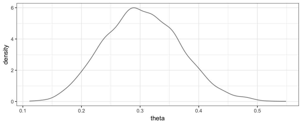

simple_mcmc <- as.matrix(simple_stanfit)
mcmc_areas(simple_mcmc, prob = 0.9, pars = "theta")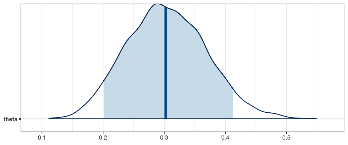

mcmc_areas(as.mcmc.list(simple_stanfit), prob = 0.9, pars = "theta")

diag_mcmc(as.mcmc.list(simple_stanfit))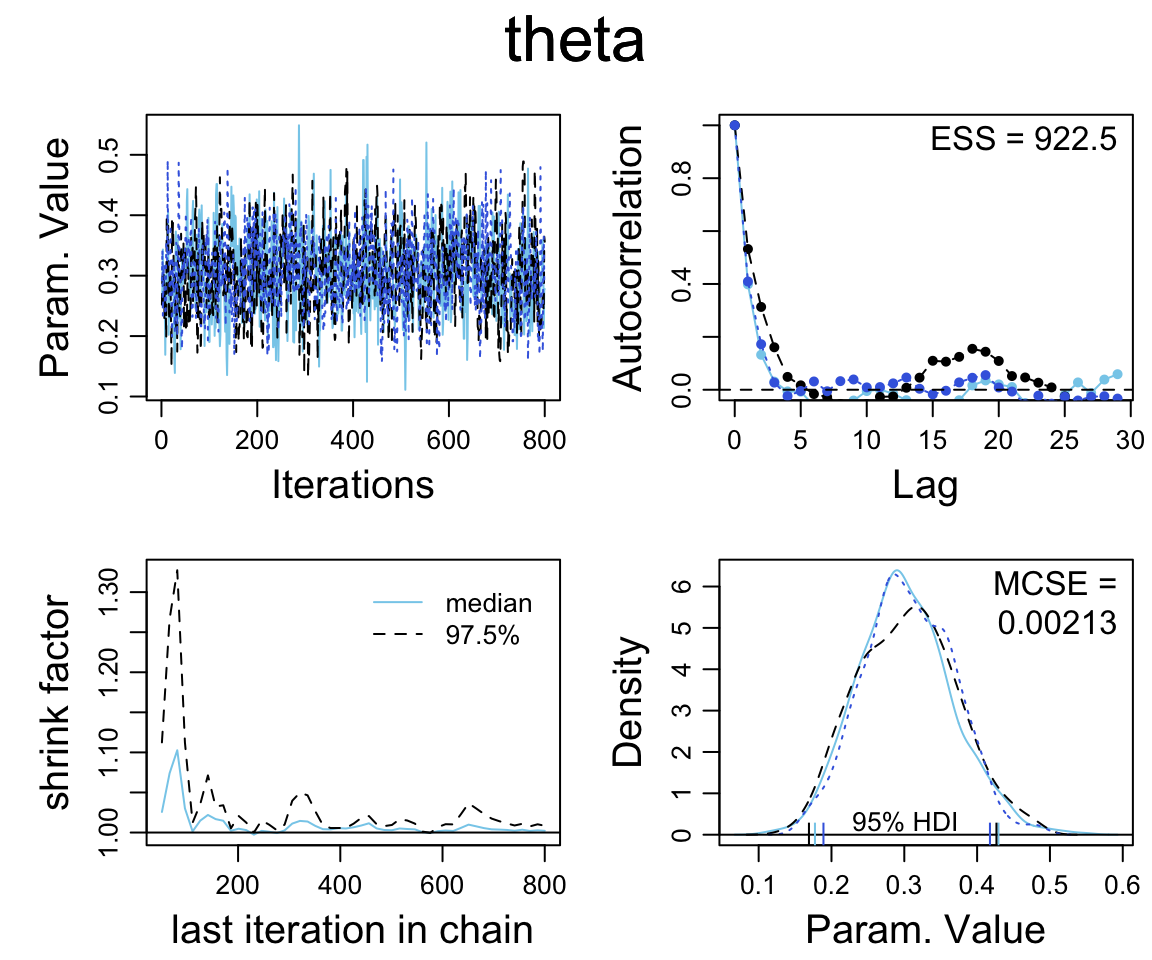

14.3 Samping from the prior

In JAGS, to sample from the posterior, we just “removed the data”. For any parameter values, the likelihood of not having any data if we don’t collect any data is 1. So the posterior is the same as the prior.

Unlike JAGS, Stan does not allow missing data, so we need a different way to sample from the posterior. In Stan, we will remove the likelihood. To understand why this works, let’s think a little bit about how Stan operates.

All internal work is done on the log scale.

log prior, log likelihood, log posterior.
Additive constants on the log scale (multiplicative constants on the natural scale) don’t matter…

… at least not for generating posterior samples, so they can be ignored or chosen conveniently. The distribution functions in Stan are really logs of kernels with constants chosen to optimize efficiency of computation.
log(posterior) = log(prior) + log(likelihood) + constant

So if we don’t add in the likelihood part, we just get the prior again as the posterior.

A line like

y ~ bernoulli(theta);

Is just telling stan to add the log of the bernoulli pmf for each value of the data vector y using the current value for theta. If we comment out that line, no log likelihood will be added.

data {
  int<lower=0> N;  // N is a non-negative integer
  int y[N];          // y is a length-N vector of integers
}
parameters {
  real<lower=0,upper=1> theta;  // theta is between 0 and 1
} 
model {
  theta ~ beta (1,1);
  // y ~ bernoulli(theta);     // comment out to remove likelihood
}

simple0_stanfit <- 
  sampling(
    simple0_stan, 
    data  = list(
      N = 50,
      y = c(rep(1, 15), rep(0, 35))
    ),
    chains = 3,     # default is 4
    iter = 1000,    # default is 2000
    warmup = 200    # default is half of iter
  )

14.4 Exercises

Let’s compare Stan and JAGS on the therapeutic touch example from Chapter 9. (See Figure 9.7 on page 236.) Stan and JAGS code for this example are below. The data are in TherapeuticTouch.
```
data {
  int<lower=1> Nsubj;
  int<lower=1> Ntotal;
  int<lower=0,upper=1> y[Ntotal];
  int<lower=1> s[Ntotal]; // notice Ntotal not Nsubj
}
parameters {
  real<lower=0,upper=1> theta[Nsubj]; // individual prob correct
  real<lower=0,upper=1> omega;        // group mode
  real<lower=0> kappaMinusTwo;        // group concentration minus two
}
transformed parameters {
  real<lower=0> kappa;  
  kappa <- kappaMinusTwo + 2;
}
model {
  omega ~ beta(1, 1);
  kappaMinusTwo ~ gamma(1.105125, 0.1051249 );  // mode=1, sd=10 
  theta ~ beta(omega * (kappa-2) + 1, (1 - omega) * (kappa-2) + 1); 
  for ( i in 1:Ntotal ) {
    y[i] ~ bernoulli(theta[s[i]]);
  }
}
```
```
jags_model <- function() {
  for ( i in 1:Ntotal ) {
    y[i] ~ dbern( theta[s[i]] )
  }
  for (s in 1:Nsubj ) {
    theta[s] ~ dbeta(omega * (kappa-2) + 1, (1-omega) * (kappa-2) + 1) 
  }
  omega ~ dbeta(1, 1) 
  kappa <- kappaMinusTwo + 2
  kappaMinusTwo ~ dgamma(1.105125, 0.1051249)  # mode=1, sd=10 
}
```
Now answer the following questions.
1. What does the transformed parameters block of the Stan code do?
2. In the Stan code, there are two lines with ~ in them. One is inside a for loop and the other not. Why?
3. Compile the Stan program, and note how long it takes.
4. Now generate posterior samples using both the JAGS and Stan versions. Do the produce the same posterior distribution? How do the effective sample sizes compare?
5. Tweak the settings until you get similar effective sample sizes and rhat values from both Stan and JAGS. (ESS is the best metric of how much work they have done, and we want to be sure both algorithms think they are converging to get a fair comparison.) Once you have done that, compare their speeds. Which is faster in this example? By how much? (If you want R to help automate the timing, you can use system.time().)