21 Dichotymous Response
21.1 What Model?
Let’s suppose we want to predict a person’s gender from their height and weight. What sort of model should we use? Give a particular height and weight, a person might be male or female. So for a given height/weight combination, the distribution of gender is a Bernoulli random variable. Our goal is to convert the height/weight combination into the parameter \(\theta\) specifying what proportion of people with that height and weign combination are male (or female).
So our model looks something like
\[\begin{align*} Y &\sim {\sf Bern}(\theta) \\ \theta &= \mathrm{f}(\texttt{height}, \texttt{weight}) \end{align*}\]
But what functions should we use for \(f\)?
21.1.1 A method with issues: Linear regression
One obvious thing to try is a linear function:
\[\begin{align*} Y &\sim {\sf Bern}(\theta) \\ \theta &= \beta_0 + \beta_{\texttt{height}} \texttt{height} + \beta_{\texttt{weight}} \texttt{weight} \end{align*}\]
An interaction term could easily be added as well. This model is basically converting the dichotymous response into a quantitative variable (0’s and 1’s) and using the same sort of regression model we have used for metric variables, but with a different noise distribution.
One problem with this model is that our linear function might well return values outside the interval \([0, 1]\). This would cause two problems:
- It is making a prediction we know is incorrect.
- The Bernoulli random variable needs a value of \(\theta\) between 0 and 1, so our likelihood function would be broken.
This model is still sometimes use (but with normal noise rather than Bernoulli noise to avoid breaking the likelihood function). But there are better approaches.
21.1.2 The usual approach: Logistic regression
We would like to use a linear function, but convert its range from \((-\infty, \infty)\) to \((0, 1)\). Alternatively, we can convert the the range \((0,1)\) to \((-\infty, \infty)\) and parameterize the Bernoulli distribution differently.
The most common transformation used the log odds transformation: \[ \begin{array}{rcl} \mathrm{probability} & \theta & (0, 1) \\ \mathrm{odds} & \theta \mapsto \frac{\theta}{1- \theta} & (0, \infty) \\ \mathrm{log\ odds} & \theta \mapsto \log(\frac{\theta}{1- \theta}) & (-\infty, \infty) \\ \end{array} \]
Read backwards, this is the logistic transformation
\[\begin{array}{rcl} \mathrm{log\ odds} & x & (-\infty, \infty) \\ \mathrm{odds} & x \mapsto e^x & (0, \infty) \\ \mathrm{probability} & x \mapsto \frac{e^x}{1 + e^x} & (0, 1) \\ \end{array}\]These functions are available via the mosaic packge as logit() and ilogit():
logit## function(x)
## {
## log(x/(1 - x))
## }
## <bytecode: 0x7f94920e55f0>
## <environment: namespace:mosaicCore>ilogit## function (x)
## {
## exp(x)/(1 + exp(x))
## }
## <bytecode: 0x7f9491bdd618>
## <environment: namespace:mosaicCore>The inverse logit function is also called the logistic function and the logistic regression model is
\[\begin{align*} Y &\sim {\sf Bern}(\theta) \\ \theta &= \mathrm{logistic}(\beta_0 + \beta_{\texttt{height}} \texttt{height} + \beta_{\texttt{weight}} \texttt{weight}) \\ \mathrm{logit}(\theta) &= \beta_0 + \beta_{\texttt{height}} \texttt{height} + \beta_{\texttt{weight}} \texttt{weight} \end{align*}\]
The logit function is called the link function and the logistic function is the inverse link function.
21.1.3 Other approaches
We could do a similar thing with any pair of functions that convert back and forth between \((0,1)\) and \((-\infty, \infty)\). For any random variable, the cdf (cumulative distribution function) has domain \((-\infty, \infty)\) and range \((0,1)\), so
- Any cdf/inverse cdf pair can be used in place of the logistic tranformation.
- using
pnorm()andqnorm()is called **probit regression*.
- using
- We can also work this backwards and create a random variable that has the logistic function as its cdf. The random variable is called (wait for it) the logistic random variable.
gf_function(ilogit, xlim = c(-6, 6), color = ~"logistic") %>%
  gf_function(pnorm, color = ~"probit (standard)") %>%
  gf_function(pnorm, args = list(sd = 1.8),
              color = ~"probit (mean = 0, sd = 1.8)") %>%
  gf_theme(legend.position = "top") %>%
  gf_labs(color = "")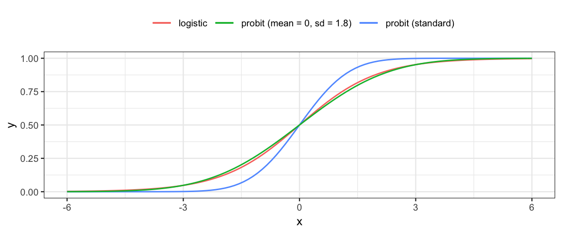
21.1.4 Preparing the data
We will use a subset of the NHANES data for this example.
This is a different data set from the example in the book (which uses
synthetic data). Since the data there are in pounds and inches, we’ll convert
the NHANES data to these units.
As in other models, we need to convert our dichotymous variable into 0’s and 1’s.
We certainly want to remove children from the model since height and weight patterns
are different for children and adults. In fact, we’ll just select
out the 22-year-olds.
While we are at it, we’ll get rid of the variables we don’t need and remove
any rows with missing values in those three rows.
library(NHANES)
library(brms)
nhanes <-
  NHANES %>%
  mutate(
    weight = Weight * 2.2,
    height = Height / 2.54,
    male = as.numeric(NHANES$Gender == "male"),
  ) %>%
  filter(Age == 22) %>%
  select(male, height, weight) %>%
  filter(complete.cases(.))  # remove rows where any of the 3 variables is missing
21.1.5 Specifying family and link function in brm()
Compared to our usual linear regression model, we need to make two adjustments:
- Use the Bernoulli family of distriutions for the noise
- Use the logit link (logistic inverse link) function to translate back and forth between the linear part of the model and the distribution.
Both are done simultaneously when we set the family argument in brm(). Each
family comes with a default link function, but we can override that if we like.
So for logistic and probit regression, we use
logistic_brm <-
  brm(male ~ height + weight, family = bernoulli(link = logit), data = nhanes)
## Compiling the C++ model## Start samplingprobit_brm <-
brm(male ~ height + weight, family = bernoulli(link = probit), data = nhanes)## Compiling the C++ model## Start samplingThe rest of the model behaves as before. In particular, a t-distribution is used for the intercept and improper uniform distributions are used for the other regression coefficients. This model doesn’t have a \(\sigma\) parameter. (The variance of a Bernoulli distribution is determined by the probability parameter.)
prior_summary(logistic_brm)| prior | class | coef | group | resp | dpar | nlpar | bound |
|---|---|---|---|---|---|---|---|
| b | |||||||
| b | height | ||||||
| b | weight | ||||||
| student_t(3, 0, 10) | Intercept |
21.2 Interpretting Logistic Regression Models
Beore getting our model with two predictors, let’s look at a model with only one predictor.
male_by_weight_brm <-
  brm(male ~ weight, family = bernoulli(), data = nhanes)
## Compiling the C++ model## recompiling to avoid crashing R session## Start samplingmale_by_weight_brm## Family: bernoulli
## Links: mu = logit
## Formula: male ~ weight
## Data: nhanes (Number of observations: 135)
## Samples: 4 chains, each with iter = 2000; warmup = 1000; thin = 1;
## total post-warmup samples = 4000
##
## Population-Level Effects:
## Estimate Est.Error l-95% CI u-95% CI Eff.Sample Rhat
## Intercept -2.12 0.82 -3.78 -0.58 3545 1.00
## weight 0.01 0.00 0.00 0.02 3499 1.00
##
## Samples were drawn using sampling(NUTS). For each parameter, Eff.Sample
## is a crude measure of effective sample size, and Rhat is the potential
## scale reduction factor on split chains (at convergence, Rhat = 1).mcmc_combo(as.mcmc.list(stanfit(male_by_weight_brm)))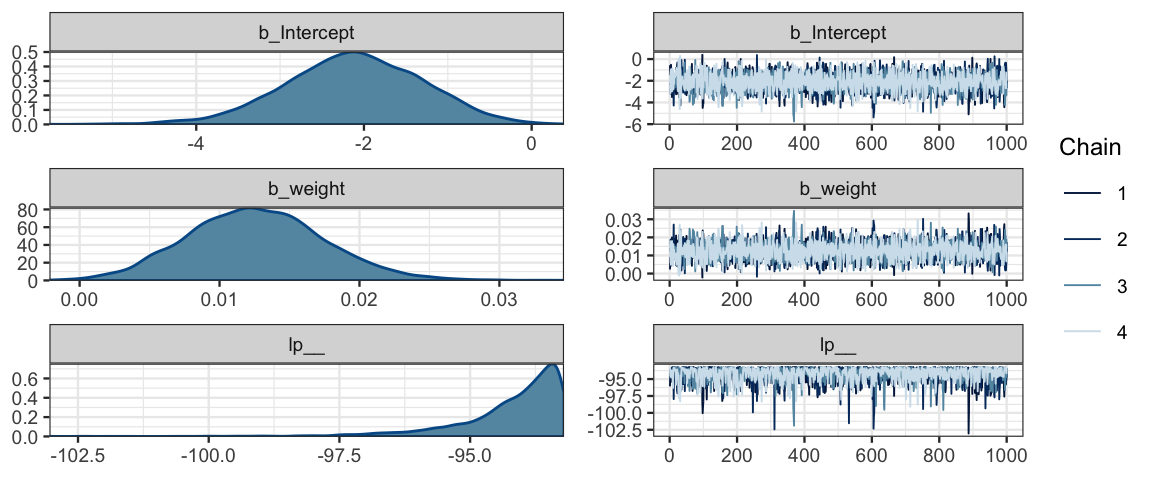
plot_post(posterior(male_by_weight_brm)$b_weight)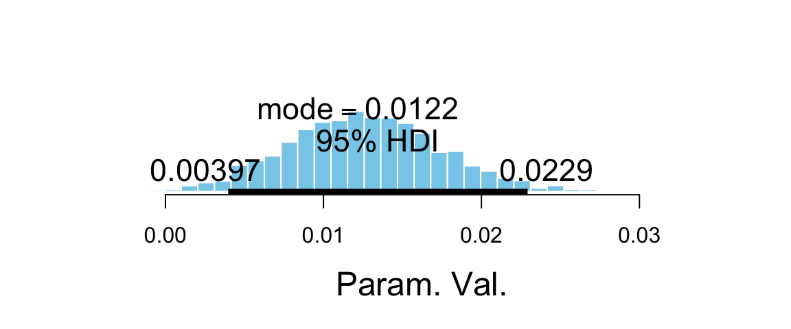
## $posterior
##       ESS    mean  median    mode
## var1 3459 0.01261 0.01246 0.01218
##
## $hdi
##   prob      lo      hi
## 1 0.95 0.00397 0.02292
p <- marginal_effects(male_by_weight_brm) %>% plot(plot = FALSE)
p$weight %>%
gf_jitter(male ~ weight, data = nhanes, inherit = FALSE,
width = 0, height = 0.03, alpha = 0.3)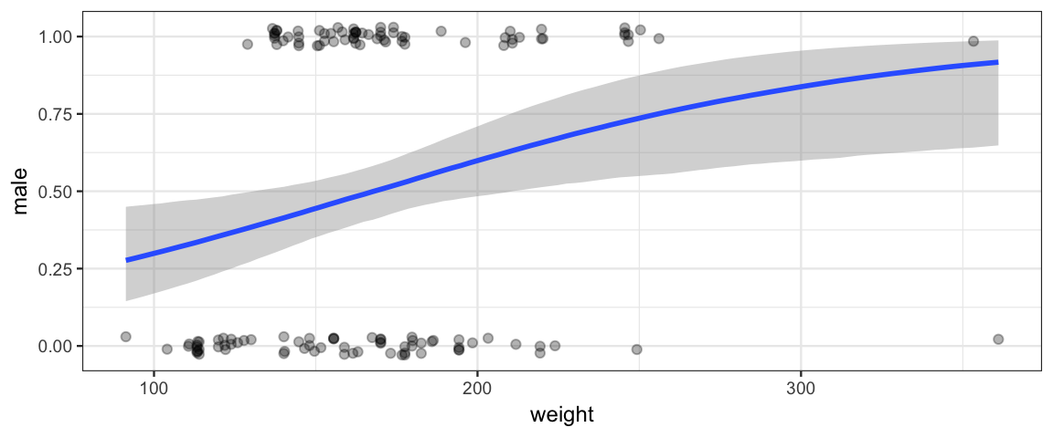
Things we learn from this model:
There is clearly a upward trend – heavier people are more likely to be male than lighter people are. This is seen in the posterior distribution for \(\beta_{\mathrm{weight}}\).
hdi(posterior(male_by_weight_brm), pars = "b_weight")par lo hi mode prob b_weight 0.004 0.0229 0.0123 0.95 The rise is gentle, not steep. There is no weight at which we abruptly believe gender is much more likely to be male above that weight and female below that weight.
For a given value of \(\theta = \langle \beta_0, \beta_{\mathrm{weight}}\rangle\) we can compute the weight at which the model believes the gender split is 50/50. Probability is 0.5 when the odds is 1 and the log odds is 0. And \(\beta_0 + \beta_{\mathrm{weight}} \mathrm{weight} = 0\) when \(\mathrm{weight} = -\beta_0 / \beta_{\mathrm{weight}}\). A 95% HDI For this value is quite wide.
Post <-
  posterior(male_by_weight_brm) %>%
  mutate(fifty_fifty = - b_Intercept / b_weight)
h <- hdi(Post, pars = "fifty_fifty"); h
par lo hi mode prob fifty_fifty 126.6 204.3 172.6 0.95 p$weight %>% gf_segment(0.5 + 0.5 ~ lo + hi, data = h, color = "red", inherit = FALSE)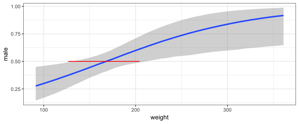
logistic_brm## Family: bernoulli
## Links: mu = logit
## Formula: male ~ height + weight
## Data: nhanes (Number of observations: 135)
## Samples: 4 chains, each with iter = 2000; warmup = 1000; thin = 1;
## total post-warmup samples = 4000
##
## Population-Level Effects:
## Estimate Est.Error l-95% CI u-95% CI Eff.Sample Rhat
## Intercept -64.73 10.86 -87.60 -45.91 3159 1.00
## height 0.95 0.16 0.67 1.28 3223 1.00
## weight 0.01 0.01 -0.01 0.02 3696 1.00
##
## Samples were drawn using sampling(NUTS). For each parameter, Eff.Sample
## is a crude measure of effective sample size, and Rhat is the potential
## scale reduction factor on split chains (at convergence, Rhat = 1).21.3 Robust Logistic Regression
For models with metric response, using t distribuitons instead of normal distributions made the models more robust (less influenced by unusually large or small values in the data).
Logistic regression can also be strongly influenced by unusual observations. In our example, if there is an unusually heavy woman or an unusually light man, the likelihood will be very small unless we flatten the logistic curve. But we cannot simply replace a normal distribution with a t distribution because our likelihood does not involve a normal distribution.
Kruschke recommends a methods that fits a mixture of the usual logistic regression model and a model that is “just guessing” (50-50 chance of being male or female). That Stan development folks (and others) recommend a different appraoch: Fit the model with an inverse t cdf. This is like a probit model, but with more flexibility. In particular, if the degrees of freedom is small, the inverse t cdf will approach its assymptotes more slowly than the probit or logistic models do.
Getting brm() to fit this model requires a few extra steps:
- define the inverse t cdf function using
stanvars - use an identity link (since we will be coding in the link/inverse link manually).
- turn off linear model evaluation of the main formula with
nl = TRUE. (This can be used for other non-linear model situations as well.)
# define inverse robit function (Stan syntax)
stan_inv_robit <- "
  real inv_robit(real y, real nu) {
    return student_t_cdf(y, nu, 0, (nu - 2) / nu);
  }
"
bform <- bf(
  male ~ inv_robit(theta, nu),
  # non-linear -- use algebra as is in *main* formula
  nl = TRUE,
  # theta = theta_Intercept + theta_weight * weight + theta_height * height
  theta ~ weight + height,
  nu ~ 1,            # nu = nu_Intercept (ie. just one value of nu)
  family = bernoulli("identity")           # identity link function
)

bprior <-
  prior(normal(0, 5), nlpar = "theta") +
  prior(gamma(2, 0.1), nlpar = "nu", lb = 2)

robit_brm <-
  brm(bform, prior = bprior, data = nhanes,
      stanvars = stanvar(scode = stan_inv_robit, block = "functions")
  )
## Compiling the C++ model## Start sampling## Warning: There were 3 transitions after warmup that exceeded the maximum treedepth. Increase max_treedepth above 10. See
## http://mc-stan.org/misc/warnings.html#maximum-treedepth-exceeded## Warning: Examine the pairs() plot to diagnose sampling problemsprior_summary(robit_brm)
robit_brm
loo(robit_brm, reloo = TRUE)
loo(logistic_brm, reloo = TRUE)new_data <- expand.grid(
height = seq(60, 75, by = 3),
weight = seq(125,225, by = 25)
)
bind_cols(
new_data,
data.frame(predict(logistic_brm, newdata = new_data, transform = ilogit))
)| height | weight | Estimate | Est.Error | Q2.5 | Q97.5 |
|---|---|---|---|---|---|
| 60 | 125 | 0.5006 | 0.0121 | 0.5000 | 0.5000 |
| 63 | 125 | 0.5051 | 0.0341 | 0.5000 | 0.5000 |
| 66 | 125 | 0.5631 | 0.1030 | 0.5000 | 0.7311 |
| 69 | 125 | 0.6947 | 0.0841 | 0.5000 | 0.7311 |
| 72 | 125 | 0.7275 | 0.0283 | 0.7311 | 0.7311 |
| 75 | 125 | 0.7307 | 0.0097 | 0.7311 | 0.7311 |
| 60 | 150 | 0.5006 | 0.0115 | 0.5000 | 0.5000 |
| 63 | 150 | 0.5069 | 0.0394 | 0.5000 | 0.7311 |
| 66 | 150 | 0.5741 | 0.1079 | 0.5000 | 0.7311 |
| 69 | 150 | 0.7023 | 0.0763 | 0.5000 | 0.7311 |
| 72 | 150 | 0.7284 | 0.0246 | 0.7311 | 0.7311 |
| 75 | 150 | 0.7308 | 0.0073 | 0.7311 | 0.7311 |
| 60 | 175 | 0.5003 | 0.0082 | 0.5000 | 0.5000 |
| 63 | 175 | 0.5098 | 0.0466 | 0.5000 | 0.7311 |
| 66 | 175 | 0.5835 | 0.1110 | 0.5000 | 0.7311 |
| 69 | 175 | 0.7069 | 0.0707 | 0.5000 | 0.7311 |
| 72 | 175 | 0.7289 | 0.0221 | 0.7311 | 0.7311 |
| 75 | 175 | 0.7309 | 0.0052 | 0.7311 | 0.7311 |
| 60 | 200 | 0.5007 | 0.0126 | 0.5000 | 0.5000 |
| 63 | 200 | 0.5113 | 0.0499 | 0.5000 | 0.7311 |
| 66 | 200 | 0.5964 | 0.1139 | 0.5000 | 0.7311 |
| 69 | 200 | 0.7119 | 0.0638 | 0.5000 | 0.7311 |
| 72 | 200 | 0.7296 | 0.0186 | 0.7311 | 0.7311 |
| 75 | 200 | 0.7309 | 0.0052 | 0.7311 | 0.7311 |
| 60 | 225 | 0.5014 | 0.0178 | 0.5000 | 0.5000 |
| 63 | 225 | 0.5136 | 0.0543 | 0.5000 | 0.7311 |
| 66 | 225 | 0.6095 | 0.1154 | 0.5000 | 0.7311 |
| 69 | 225 | 0.7133 | 0.0615 | 0.5000 | 0.7311 |
| 72 | 225 | 0.7297 | 0.0175 | 0.7311 | 0.7311 |
| 75 | 225 | 0.7310 | 0.0037 | 0.7311 | 0.7311 |
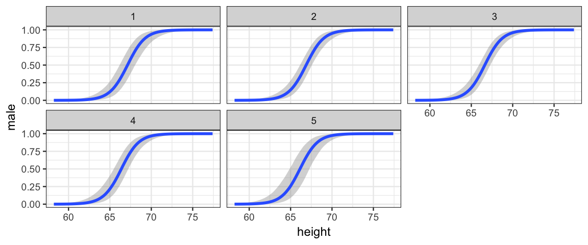
marginal_effects(
  logistic_brm, effects = "height",
  conditions = data.frame(weight = seq(125, 225, by = 25)))