13 Goals, Power, Sample Size
13.1 Intro
13.1.1 Goals
Kruschke (bold added):
Any goal of research can be formally expressed in various ways. In this chapter I will focus on the following goals formalized in terms of the highest density interval (HDI):
- Goal: Reject a null value of a parameter.
Formal expression: Show that a region of practical equivalence (ROPE) around the null value excludes the posterior 95% HDI.- Goal: Affirm a predicted value of a parameter.
Formal expression: Show that a ROPE around the predicted value includes the posterior 95% HDI.- Goal: Achieve precision in the estimate of a parameter.
Formal expression: Show that the posterior 95% HDI has width less than a specified maximum.
13.1.2 Obstacles
The crucial obstacle to the goals of research is that a random sample is only a probabilistic representation of the population from which it came. Even if a coin is actually fair, a random sample of flips will rarely show exactly 50% heads. And even if a coin is not fair, it might come up heads 5 times in 10 flips. Drugs that actually work no better than a placebo might happen to cure more patients in a particular random sample. And drugs that truly are effective might happen to show little difference from a placebo in another particular random sample of patients. Thus, a random sample is a fickle indicator of the true state of the underlying world. Whether the goal is showing that a suspected value is or isn’t credible, or achieving a desired degree of precision, random variation is the researcher’s bane. Noise is the nemesis.
13.2 Power
Because of random noise, the goal of a study can be achieved only probabilistically. The probability of achieving the goal, given the hypothetical state of the world and the sampling plan, is called the power of the planned research.
13.2.1 Three ways to increase power
Reduce measurement noise as much as possible.
We can avoid sources of variability by controlling them (keep them constant for all observational units) or by including them as co-variates inour model.
“Reduction of noise and control of other influences is the primary reason for conducting experiments in the lab instead of in the maelstrom of the real world.” (But with the downside that lab conditions might not accurately reflect the conditions of the situation we are actually interested in.)
Amplify the underlying magnitude of the effect if we possibly can.
Exmples: In a study of methods to improve reading performance, we might select participants who are reading below grade level and so have the most room to improve. When administering a drug, a larger dose is likely to show a larger effect (within reason – we don’t want undo side effects).
Increase sample size.
In principle, more data means more information and less variability. In practice, more data means more costs (time, money, etc.).
13.3 Calculating Power: 3 step process
We can calculate the power of our study by repeating the following three steps many times:
Sample parameters from a hypothetical distribution of parameter values.
These are chosen to reflect some situation we are interested in. Our main question will be “How likely are we to attain our goals in this situation.”
Given the sampled parameter values, simulate a data set (using the data collection method proposed for the study).
Using the data set, compute the posterior HDI (or some other measure related to our goal).
Each HDI can be classified as achieving or not achieving the goal. The proportion of simulated data sets that achieve the goal is our estimate of power, given the hypothesized distribution of parameter values.
13.4 Power Examples
13.4.1 Example: Catching an unfair coin
Let’s go through these steps to estimate the power of detecting a coin that comes up heads 65% of the time using a ROPE of (0.49, 0.51). Our goal in this case is an HDI that is either below 0.49 or above 0.51.
13.4.1.1 Sample parameters
In this case, this is pretty boring since our hypothetical situation is that the proportion is exactly 0.65. But for the sake of what is to come, we will create a little function to compute 0.65 for us. To improve output formatting, and so things generalize later, we will return that value as a named vector. (A data frame or list would also work.)
We can test it out by “doing” it 3 times.
library(mosaic)              # mosaic contains the do() function
draw_theta <- function() { c(theta = 0.65) }
do(3) * draw_theta()| theta |
|---|
| 0.65 |
| 0.65 |
| 0.65 |
13.4.1.2 Simulate data
For a given parameter value, we need to simulate data, in this case a number of heads and a number of flips. In our example, the number of flips is always the same, but we could design the study differently so that the number of flips was not always the same, for example by flipping until we see a certain number of heads (or tails, or both). We will make this an argument to our function so we can explore different sample sizes later.
simulate_data <-
  function(theta, n) {
    x <- rbinom(1, n, theta)
    data.frame(theta = theta, heads = x, flips = n)
  }
do(3) * simulate_data(0.60, 100)| theta | heads | flips | .row | .index |
|---|---|---|---|---|
| 0.6 | 58 | 100 | 1 | 1 |
| 0.6 | 61 | 100 | 1 | 2 |
| 0.6 | 56 | 100 | 1 | 3 |
13.4.1.3 Compute the HDI
From our simulated data, we need to compute and HDI. To avoid needing to simulate, we will use what we know about beta distributions to compute the posterior distribution analytically. To keep the code simple, we will use a central 95% interval that is not an HDI, but it should be close.
The default prior is uniform (\({\sf Beta}(1,1)\)), but we will allow arguments to the function that let us experiment with different priors as well.
compute_hdi <- function(data, prior = list(a = 1, b = 1)) {
  # posterior
  post <- data.frame(a = prior$a + data$heads, b = prior$b + data$flips - data$heads)
  # not quite the HDI
  data.frame(
    theta = data$theta,
    x = data$heads,
    n = data$flips,
    lo = qbeta(0.025, post$a, post$b),
    hi = qbeta(0.975, post$a, post$b)
  )
}
draw_theta() %>%
  simulate_data(n = 100) %>%
compute_hdi()| theta | x | n | lo | hi |
|---|---|---|---|---|
| 0.65 | 61 | 100 | 0.5118 | 0.6999 |
13.4.1.4 Lather, rinse, repeat
Now we repeat these three steps many times.
do(5) * {
  draw_theta() %>%
    simulate_data(n = 100) %>%
    compute_hdi()
}| theta | x | n | lo | hi | .row | .index |
|---|---|---|---|---|---|---|
| 0.65 | 69 | 100 | 0.5934 | 0.7722 | 1 | 1 |
| 0.65 | 70 | 100 | 0.6039 | 0.7810 | 1 | 2 |
| 0.65 | 64 | 100 | 0.5421 | 0.7273 | 1 | 3 |
| 0.65 | 59 | 100 | 0.4918 | 0.6814 | 1 | 4 |
| 0.65 | 67 | 100 | 0.5728 | 0.7544 | 1 | 5 |
Sims100 <-
  do(5000) * {
    draw_theta() %>%
      simulate_data(n = 100) %>%
      compute_hdi()
  }
Sims100 <-
  Sims100 %>% mutate(reject = (hi < 0.49) | (lo > 0.51))
df_stats(~reject, data = Sims100, props, counts)| prop_FALSE | prop_TRUE | n_FALSE | n_TRUE |
|---|---|---|---|
| 0.169 | 0.831 | 845 | 4155 |
The power increases if we incrase the sample size.
Sims200 <-
  do(5000) * {
    draw_theta() %>%
      simulate_data(n = 200) %>%
      compute_hdi()
  }
Sims200 <-
  Sims200 %>%  mutate(reject = (hi < 0.49) | (lo > 0.51))

df_stats(~reject, data = Sims200, props, counts)| prop_FALSE | prop_TRUE | n_FALSE | n_TRUE |
|---|---|---|---|
| 0.0166 | 0.9834 | 83 | 4917 |
13.4.2 Example: Estimating a Proportion
Suppose we would like to estimate a proportion within \(\pm 2\)%. Further suppose we have no idea what that proportion is. So now we will draw values of \(\theta\) from a uniform distribution.
13.4.2.1
draw_theta_unif <- function(a = 0, b = 1) { c(theta = runif(1, a, b)) }
do(3) * draw_theta_unif()| theta |
|---|
| 0.7242 |
| 0.9703 |
| 0.8775 |
Sims200p <-
  do(5000) * {
    draw_theta_unif() %>%
      simulate_data(n = 200) %>%
      compute_hdi()
  }
Sims200p <-
  Sims200p %>%
  mutate(
    width = hi - lo,
    success = width < 0.02)

df_stats(~ success, data = Sims200p, props, counts)| prop_FALSE | prop_TRUE | n_FALSE | n_TRUE |
|---|---|---|---|
| 0.9878 | 0.0122 | 4939 | 61 |
So a sample of size 200 isn’t going to do it (at least not very often). Let’s try 2000.
Sims2000p <-
  do(5000) * {
    draw_theta_unif() %>%
      simulate_data(n = 2000) %>%
      compute_hdi()
  }
Sims2000p <-
  Sims2000p %>%
  mutate(
    width = (hi - lo),
    center = lo + width / 2,
    success = width < 0.02)

df_stats( ~ success, data = Sims2000p, props, counts)| prop_FALSE | prop_TRUE | n_FALSE | n_TRUE |
|---|---|---|---|
| 0.8888 | 0.1112 | 4444 | 556 |
Better, but we’re still hitting our target only 10% of the time.
Sims8kp <-
  do(5000) * {
    draw_theta_unif() %>%
      simulate_data(n = 8000) %>%
      compute_hdi()
  }
Sims8kp <-
  Sims8kp %>%
  mutate(
    width = (hi - lo),
    center = lo + width / 2,
    success = width < 0.02)

df_stats( ~ success, data = Sims8kp, props, counts)| prop_FALSE | prop_TRUE | n_FALSE | n_TRUE |
|---|---|---|---|
| 0.4062 | 0.5938 | 2031 | 2969 |
We can find out a bit more about what is going on here by comparing the width of the interval to the simulate value of \(\theta\).
gf_point(width ~ theta, data = Sims8kp, shape = 21) %>%
  gf_hline(yintercept =  0.02, color = "red")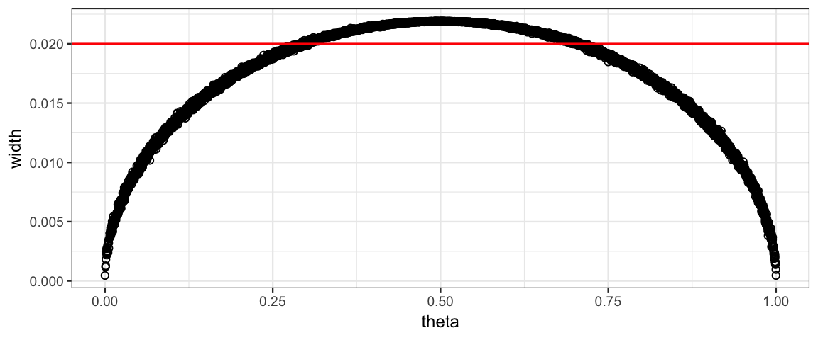
As we see, the width of the interval is wider when \(\theta\) is near 0.5. This means we can get by with a smaller sample size if we have good reason to expect that \(\theta\) is near 0 or 1. And we will need a larger sample size if we expect \(\theta\) is near 0.5.
Sims_small_theta <-
  do(5000) * {
    draw_theta_unif(0,0.2) %>%
      simulate_data(n = 3000) %>%
      compute_hdi()
  }

Sims_small_theta <-
  Sims_small_theta %>%
  mutate(
    width = hi - lo,
    success = width < 0.02
  )

df_stats(~success, data = Sims_small_theta, props, counts)| prop_FALSE | prop_TRUE | n_FALSE | n_TRUE |
|---|---|---|---|
| 0.5712 | 0.4288 | 2856 | 2144 |
gf_histogram(~ width, data = Sims_small_theta, bins = 40)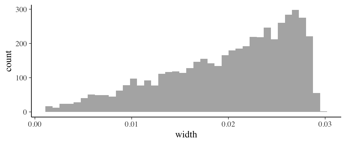
gf_point(width ~ theta, data = Sims_small_theta, shape = 21)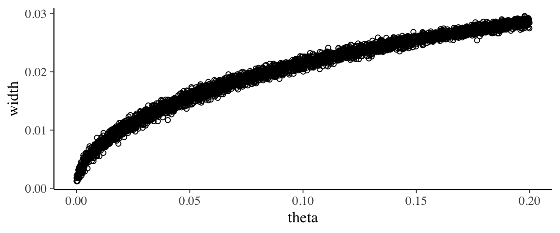
13.4.3 More Complex Example
The one proportion example is as simple as it gets
- only one parameter (the proportion)
- simple distribution (Bernoulli)
- relatively easy to come up with hypothetical distributions
- easy calculation of the posterior distribution
In a typical situation, none of these special aspects will hold. Let’s try something just one step more complex: a simple linear model.
draw_theta_slr <- function() {
  data.frame(intercept = runif(1, 10, 12),
             slope = runif(1, 3, 4),
             sigma = runif(1, 4, 5)
  )
}

do(3) * draw_theta_slr()| intercept | slope | sigma | .row | .index |
|---|---|---|---|---|
| 11.47 | 3.508 | 4.108 | 1 | 1 |
| 10.77 | 3.732 | 4.790 | 1 | 2 |
| 10.72 | 3.047 | 4.114 | 1 | 3 |
simulate_data_slr <-
  function(theta = list(slope = 1, intercept = 0, sigma = 1), n = 40, xlim = c(0,1)) {
    tibble(
      x = runif(n, xlim[1], xlim[2]),
      y = theta$intercept + theta$slope * x + rnorm(n, 0, theta$sigma)
    )
  }

gf_point(y ~ x, data = simulate_data_slr())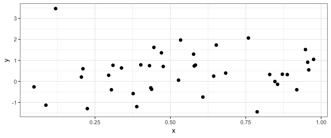
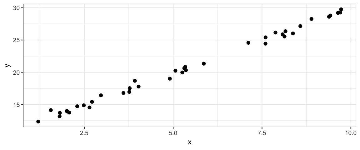
gf_point(y ~ x,
         data = simulate_data_slr(
           xlim = c(0,10),
           theta = list(slope = 2, intercept = 10, sigma = 0.5))
)
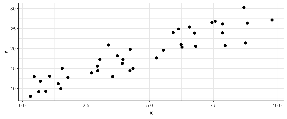
gf_point(y ~ x,
         data = simulate_data_slr(
           xlim = c(0,10),
           theta = list(slope = 2, intercept = 10, sigma = 2.5))
)
slr_model <- brm( y ~ x, data = simulate_data_slr())## Compiling the C++ model## Start samplingcompute_hdi_slr <-
function(data) {
model <- update(slr_model, newdata = data)
model %>% posterior() %>% hdi()
}draw_theta_slr() %>%
simulate_data_slr() %>%
compute_hdi_slr()## Start samplingLet’s do 100 simulations. This is going to require posterior sampling from 100
models, so we want to be confident things are working properly before we simulate
thousands of these. The use of update() will make this run much faster.
Sims_slr <-
do(100) * {
draw_theta_slr() %>%
  simulate_data_slr() %>%
  compute_hdi_slr()
}## Start sampling
## Start sampling
## Start sampling
## Start sampling
## Start sampling
## Start sampling
## Start sampling
## Start sampling
## Start sampling
## Start sampling
## Start sampling
## Start sampling
## Start sampling
## Start sampling
## Start sampling
## Start sampling
## Start sampling
## Start sampling
## Start sampling
## Start sampling
## Start sampling
## Start sampling
## Start sampling
## Start sampling
## Start sampling
## Start sampling
## Start sampling
## Start sampling
## Start sampling
## Start sampling
## Start sampling
## Start sampling
## Start sampling
## Start sampling
## Start sampling
## Start sampling
## Start sampling
## Start sampling
## Start sampling
## Start sampling
## Start sampling
## Start sampling
## Start sampling
## Start sampling## Warning: There were 1 transitions after warmup that exceeded the maximum treedepth. Increase max_treedepth above 10. See
## http://mc-stan.org/misc/warnings.html#maximum-treedepth-exceeded## Warning: Examine the pairs() plot to diagnose sampling problems## Start sampling
## Start sampling
## Start sampling
## Start sampling
## Start sampling
## Start sampling
## Start sampling
## Start sampling
## Start sampling
## Start sampling
## Start sampling
## Start sampling
## Start sampling
## Start sampling
## Start sampling
## Start sampling
## Start sampling
## Start sampling
## Start sampling
## Start sampling
## Start sampling
## Start sampling
## Start sampling
## Start sampling
## Start sampling
## Start sampling
## Start sampling
## Start sampling
## Start sampling
## Start sampling
## Start sampling
## Start sampling
## Start sampling
## Start sampling
## Start sampling
## Start sampling
## Start sampling
## Start sampling
## Start sampling
## Start sampling
## Start sampling
## Start sampling## Warning: There were 1 transitions after warmup that exceeded the maximum treedepth. Increase max_treedepth above 10. See
## http://mc-stan.org/misc/warnings.html#maximum-treedepth-exceeded
## Warning: Examine the pairs() plot to diagnose sampling problems## Start sampling
## Start sampling
## Start sampling
## Start sampling
## Start sampling
## Start sampling
## Start sampling
## Start sampling
## Start sampling
## Start sampling
## Start sampling
## Start sampling
## Start sampling
## Start sampling
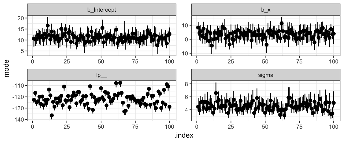
## Start samplingHere is a plot showing the simulated HDIs. For any particular goal, it would now be easy to compute how often the goal is attained.
gf_pointrange( mode + lo + hi ~ .index, data = Sims_slr) %>%
  gf_facet_wrap( ~ par, scales = "free")