4 Probability
4.1 Some terminology
Probability is about quantifying the relative chances of various possible outcomes of a random process.
As a very simple example (used to illustrate the terminology below), considering rolling a single 6-sided die.
sample space: The set of all possible outcomes of a random process. [{1, 2, 3, 4, 5, 6}]
event: a set of outcomes (subset of sample space) [E = {2, 4, 6} is the event that we obtain an even number]
probability: a number between 0 and 1 assigned to an event (really a function that assigns numbers to each event). We write this P(E). [P(E) = 1/2 where E = {1, 2, 3}]
random variable: a random process that produces a number. [So rolling a die can be considered a random variable.]
probability distribution: a description of all possible outcomes and their probabilities. For rolling a die we might do this with a table like this:
| 1 | 2 | 3 | 4 | 5 | 6 |
|---|---|---|---|---|---|
| 1/6 | 1/6 | 1/6 | 1/6 | 1/6 | 1/6 |
support (of a random variable): the set of possible values of a random variable. This is very similar to the sample space.
probability mass function (pmf): a function (often denoted with \(p\) or \(f\)) that takes possible values of a discrete random variable as input and returns the probability of that outcome.
If \(S\) is the support of the random variable, then \[ \sum_{x \in S} p(x) = 1 \] and any function with this property is a pmf.
Probabilities of events are obtained by adding the probabilities of all outcomes in the event:
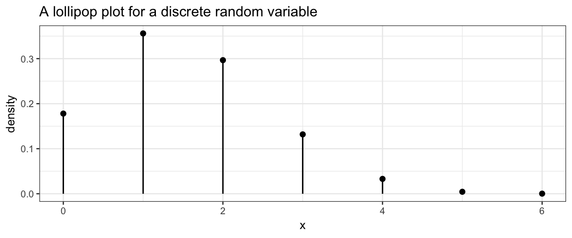
\[ \operatorname{Pr}(E) = \sum_{x \in E} p(x) \] * pmfs can be represented in a table (like the one above) or graphically with a probability histogram or lollipop plot like the ones below. [These are not for the 6-sided die, as we can tell because the probabilities are not the same for each input; the die rolling example would make very boring plots.]
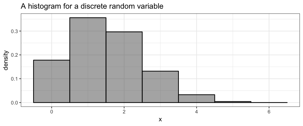
- Histograms are generally presented on the density scale so the total area of the histogram is 1. (In this example, the bin widths are 1, so this is the same as being on the probability scale.)
probability density function (pdf): a function (often denoted with \(p\) or \(f\)) that takes the possible values of continuous random variable as input and returns the probability density.
- If \(S\) is the support of the random variable, then2 \[ \int_{x \in S} f(x) \; dx = 1 \] and any function with this property is a pmf.
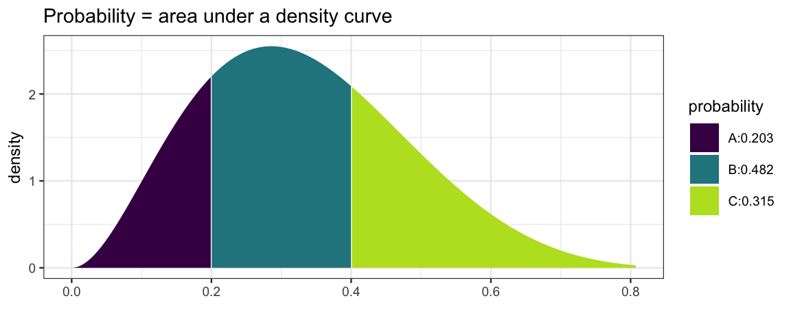
- Probabilities are obtained by integrating (visualized by the area under the density curve):
\[ \operatorname{Pr}(a \le X \le b) = \int_a^b f(x) \; dx \]
kernel function: If \(\int_{x \in S} f(x) \; dx = k\) for some real number \(k\), then \(f\) is a kernel function. We can obtain the pdf from the kernel by dividing by \(k\).
cumulative distribution function (cdf): a function (often denoted with a capital \(F\)) that takes a possible value of a random variable as input and returns the probability of obtaining a value less than or equal to the input: \[ F_X(x) = \operatorname{Pr}(X \le x) \] cdfs can be defined for both discrete and continuous random variables.
a family of distributions: is a collection of distributions which share common features but are distinguished by different parameter values. For example, we could have the family of distributions of fair dice random variables. The parameter would tell us how many sides the die has. Statisticians call this family the discrete uniform distributions because all the probabilities are equal (1/6 for 6-sided die, 1/10 for a \(D_10\), etc.).
We will get to know several important families of distributions, among them the binomial, beta, normal, and t families will be especially useful. You may already be familiar with some or all of these. We will also use distributions that have no name and are only described by a pmf or pdf, or perhaps only by a large number of random samples from which we attempt to estimate the pmf or pdf.
4.2 Distributions in R
pmfs, pdfs, and cdfs are available in R for many important families of distributions. You just need to know a few things:
- each family has a standard abbreviation in R
- pmf and pdf functions begin with the letter
dfollowed by the family abbreviation - cdf functions begin with the letter
pfollowed by the family abbreviation - the inverse of the cdf function is called a quantile function,
it starts with the letter
q - functions beginning with
rcan generate random samples from a distribution - help for any of these functions will tell you what R calls the parameters of the family.
gf_dist()can be used to make various plots of distributions.
4.2.1 Example: Normal distributions
As an example, let’s look the family of normal distributions. If you type
dnorm( and then hit TAB or if you type args(dnorm) you can see the arguments
for this function.
args(dnorm)## function (x, mean = 0, sd = 1, log = FALSE)
## NULLFrom this we see that the parameters are called mean and sd and have
default value of 0 and 1. These values will be used if we don’t specify
something else.
As with many of the pmf and pdf functions,
there is also an option to get back the log of the
pmf or pdf by setting log = TRUE. This turns out to be computationally much
more efficient in many contexts, as we will see.
Let’s begin with some pictures of a normal distribution with mean 10 and standard deviation 1:
gf_dist("norm", mean = 10, sd = 2, title = "pdf for Norm(10, 2)")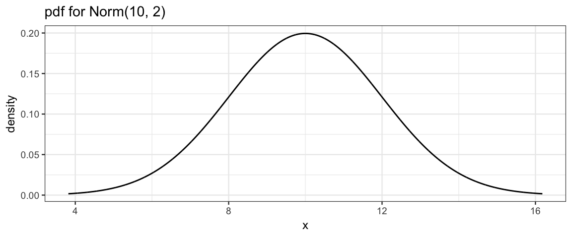
gf_dist("norm", mean = 10, sd = 2, kind = "cdf", title = "cdf for Norm(10, 2)")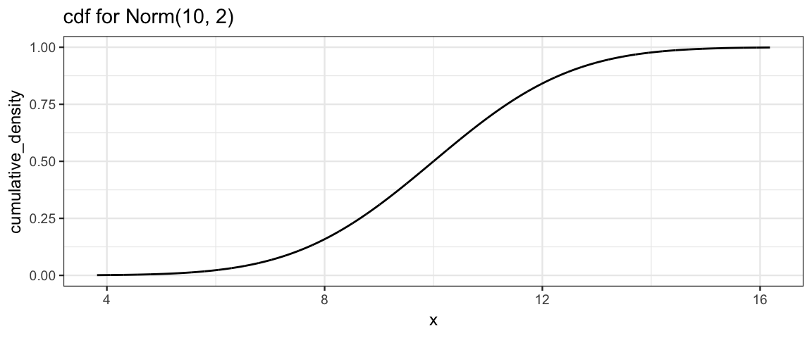
Now some exercises. Assume \(X \sim {\sf Norm}(10, 2)\).
What is \(\operatorname{Pr}(X \le 5)\)?
We can see by inspection that it is less that 0.5.
pnorm()will give us the value we are after;xpnorm()will provide more verbose output and a plot as well.
pnorm(5, mean = 10, sd = 2)## [1] 0.00621xpnorm(5, mean = 10, sd = 2)## ## If X ~ N(10, 2), then## P(X <= 5) = P(Z <= -2.5) = 0.00621## P(X > 5) = P(Z > -2.5) = 0.9938## 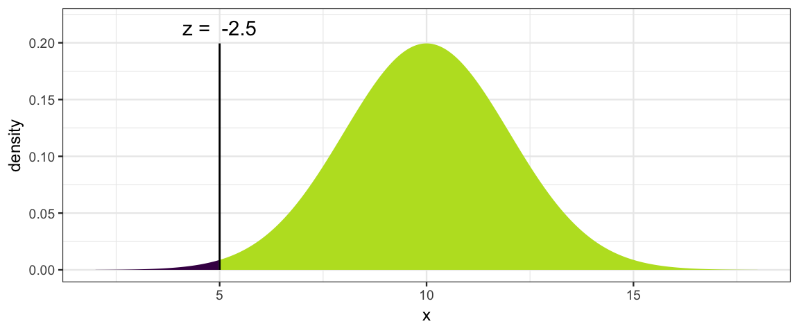
## [1] 0.00621- What is \(\operatorname{Pr}(5 \le X \le 10)\)?
pnorm(10, mean = 10, sd = 2) - pnorm(5, mean = 10, sd = 2)## [1] 0.4938How tall is the density function at it’s peak?
Normal distributions are symmetric about their means, so we need the value of the pdf at 10.
dnorm(10, mean = 10, sd = 2)## [1] 0.1995What is the mean of a Norm(10, 2) distribution?
Ignoring for the moment that we know the answer is 10, we can compute it. Notice the use of
dnorm()in the computation.
integrate(function(x) x * dnorm(x, mean = 10, sd = 2), -Inf, Inf)## 10 with absolute error < 0.0011What is the variance of a Norm(10, 2) distribution?
Again, we know the answer is the square of the standard deviation, so 4. But let’s get R to compute it in a way that would work for other distributions as well.
integrate(function(x) (x - 10)^2 * dnorm(x, mean = 10, sd = 2), -Inf, Inf)## 4 with absolute error < 7.1e-05- Simulate a data set with 50 values drawn from a \({\sf Norm}(10, 2)\) distribution and make a histogram of the results and overlay the normal pdf for comparison.
x <- rnorm(50, mean = 10, sd = 2)
# be sure to use a density histogram so it is on the same scale as the pdf!
gf_dhistogram(~ x, bins = 10) %>%
  gf_dist("norm", mean = 10, sd = 2, color = "red")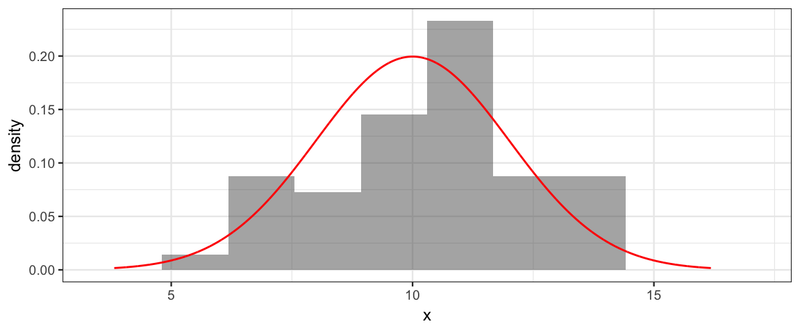
4.2.2 Simulating running proportions
library(ggformula)
library(dplyr)
theme_set(theme_bw())
Flips <-
  tibble(
    n = 1:500,
    flip = rbinom(500, 1, 0.5),
    running_count = cumsum(flip),
    running_prop  = running_count / n
  )

gf_line(
  running_prop ~ n, data = Flips,
  color = "skyblue",
  ylim = c(0, 1.0),
  xlab = "Flip Number", ylab = "Proportion Heads",
  main = "Running Proportion of Heads") %>%
  gf_hline(yintercept = 0.5, linetype = "dotted")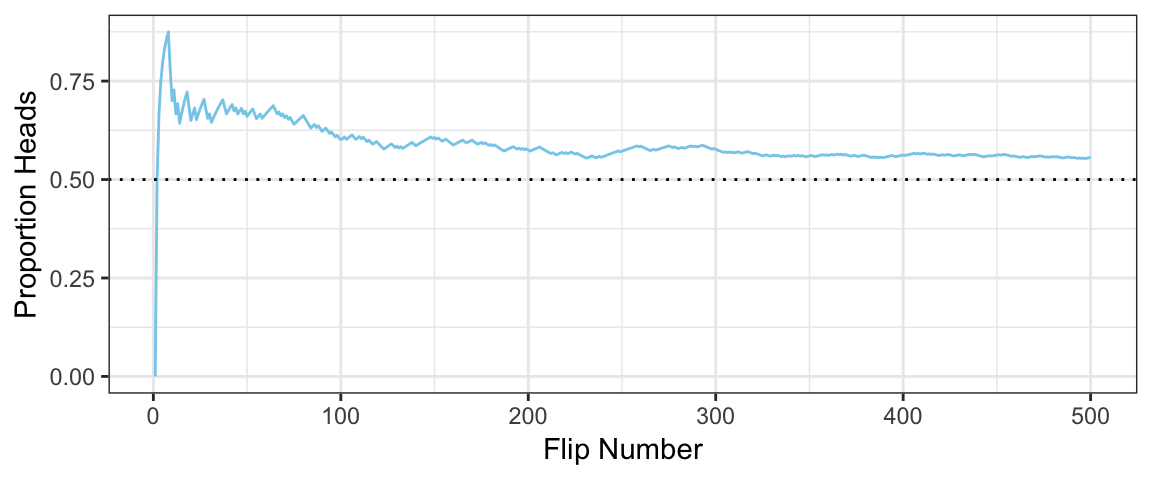
4.3 Joint, marginal, and conditional distributions
Sometimes (most of the time, actually) we are interested joint distributions. A joint distribution is the distribution of multiple random variables that result from the same random process. For example, we might roll a pair of dice and obtain two numbers (one for each die). Or we might collect a random sample of people and record the height for each of them. Or we might randomly select one person, but record multiple facts (height and weight, for example). All of these situations are covered by joint distributions.3
4.3.1 Example: Hair and eye color
Kruschke illustrates joint distributions with an example of hair and eye color recorded for a number of people.4 That table below has the proportions for each hair/eye color combination. For example,
| Hair/Eyes | Blue | Green | Hazel | Brown |
|---|---|---|---|---|
| Black | 0.034 | 0.115 | 0.008 | 0.025 |
| Blond | 0.159 | 0.012 | 0.027 | 0.017 |
| Brown | 0.142 | 0.201 | 0.049 | 0.091 |
| Red | 0.029 | 0.044 | 0.024 | 0.024 |
Each value in the table indicates the proportion of people that have a particular hair color and a particular eye color. So the upper left cell says that 3.4% of people have black hair and blue eyes (in this particular sample – the proportions will vary a lot depending on the population of interest). We will denote this as
\[ \operatorname{Pr}(\mathrm{Hair} = \mathrm{black}, \mathrm{Eyes} = \mathrm{blue}) = 0.034 \;. \] or more succinctly as \[ p(\mathrm{black}, \mathrm{blue}) = 0.034 \;. \] This type of probability is called a joint probability because it tells about the probability of both things happening.
Use the table above to do the following.
What is \(p(\mathrm{brown}, \mathrm{green})\) and what does that number mean?
Add the proportion across each row and down each column. (Record them to the right and along the bottom of the table.) For example, in the first row we get \[ 0.034 + 0.115 + 0.008 + 0.025 = 0.182 \;. \]
- Explain why \(p(\mathrm{black}) = 0.182\) is good notation for this number.
Up to round-off error, the total of all the proportions should be 1. Check that this is true.
What proportion of people with black hair have blue eyes?
This is called a conditional probability. We denote it as \(\operatorname{Pr}(\mathrm{Eyes} = \mathrm{blue} \mid \mathrm{Hair} = \mathrm{black})\). or \(p(\mathrm{blue} \mid \mathrm{black})\).
Compute some other conditional probabilities.
- \(p(\mathrm{black} \mid \mathrm{blue})\).
- \(p(\mathrm{blue} \mid \mathrm{blond})\).
- \(p(\mathrm{blond} \mid \mathrm{blue})\).
- \(p(\mathrm{brown} \mid \mathrm{hazel})\).
- \(p(\mathrm{hazel} \mid \mathrm{brown})\).
There are 32 such conditional probabilities that we can compute from this table. Which is largest? Which is smallest?
Write a general formula for computing the conditional probability \(p(c \mid r)\) from the \(p(r,c)\) values. (\(r\) and \(c\) are to remind you of rows and columns.)
Write a general formula for computing the conditional probability \(p(r \mid c)\) from the \(p(r,c)\) values.
If we have continuous random variables, we can do a similar thing. Instead of working with probability, we will work with a pdf. Instead of sums, we will have integrals.
Write a general formula for computing each of the following if \(p(x,y)\) is a continuous joint pdf.
- \(p_X(x) = p(x) =\)
- \(p_Y(y) = p(y) =\)
- \(p_{Y\mid X}(y\mid x) = p(y \mid x) =\)
- \(p_{X\mid Y}(y\mid x) = (x \mid y) =\)
We can expression both versions of conditional probability using a word equation. Fill in the missing numerator and denominator
\[ \mathrm{conditional} = \frac{\phantom{joint}}{\phantom{marginal}} \]
4.3.2 Independence
If \(p(x \mid y) = p(x)\) (conditional = marginal) for all combinations of \(x\) and \(y\), we say that \(X\) and \(Y\) are independent.
Use the definitions above to express independence another way.
Are hair and eye color independent in our example?
True or False. If we randomly select a card from a standard deck (52 cards, 13 denominations, 4 suits), are suit and denomination independent?
Create a table for two independent random variables \(X\) and \(Y\), each of which takes on only 3 possible values.
Now create a table for a different pair \(X\) and \(Y\) that are not independent but have the same marginal probabilities as in the previous exercise.
4.4 Exercises
- Suppose a random variable has the pdf \(p(x) = 6x (1-x)\) on the interval
\([0,1]\). (That means it is 0 outside of that interval.)
- Use
function()to create a function in R that is equivalent top(x). - Use
gf_function()to plot the function on the interval \([0, 1]\). - Integrate by hand to show that the total area under the pdf is 1 (as it should be for any pdf).
- Now have R compute that same integral (using
integrate()). What is the largest value of \(p(x)\)? At what value of \(x\) does it occur? Is it a problem that this value is larger than 1?
Hint: differentiation might be useful.
- Use
- Recall that
\(\operatorname{E}(X) = \int x f(x) \;dx\) for a continuous random variable with pdf \(f\) and
\(\operatorname{E}(X) = \sum x f(x) \;dx\) for a discrete random variable with pmf \(f\). (The
integral or sum is over the support of the random variable.) Compute
the expected value for the following random variables.
- \(A\) is discrete with pmf \(f(x) = x/10\) for \(x \in \{1, 2, 3, 4\}\).
\(B\) is continuous with kernel \(f(x) = x^2(1-x)\) on \([0, 1]\).
Hint: first figure out what the pdf is.
- Compute the variance and standard deviation of each of the distributions in the previous problem.
In Bayesian inference, we will often need to come up with a distribution that matches certain features that correspond to our knowledge or intuition about a situation. Find a normal distribution with a mean of 10 such that half of the distribution is within 3 of 10 (ie, between 7 and 13).
Hint: use
qnorm()to determine how many standard deviations are between 10 and 7.
School children were surveyed regarding their favorite foods. Of the total sample, 20% were 1st graders, 20% were 6th graders, and 60% were 11th graders. For each grade, the following table shows the proportion of respondents that chose each of three foods as their favorite.
From that information, construct a table of joint probabilities of grade and favorite food.
Are grade and favorite food independent? Explain how you ascertained the answer.
grade Ice cream Fruit French fries 1st 0.3 0.6 0.1 6th 0.6 0.3 0.1 11th 0.3 0.1 0.6
Three cards are placed in a hat. One is black on both sides, one is white on both sides, and the third is white on one side and black on the other. One card is selected at random from the three cards in the hat and placed on the table.
The top of the card is black.- What is the probability that the bottom is also black?
- What notation should we use for this probability?
The three cards from the previous problem are returned to the hat. Once again a card is pulled and placed on the table, and once again the top is black. This time a second card is drawn and placed on the table. The top side of the second card is white.
- What is the probability that the bottom side of the first card is black?
- What is the probability that the bottom side of the second card is black?
- What is the probability that the bottom side of both cards is black?
Pandas. Suppose there are two species of panda, A and B. Without a special blood test, it is not possible to tell them apart. But it is known that half of pandas are of each species and that 10% of births from species A are twins and 20% of births from species B are twins.
If a female panda has twins, what is the probability that she is from species A?
If the same panda later has another set of twins, what is the probability that she is from species A?
A different panda has twins and a year later gives birth to a single panda. What is the probability that this panda is from species A?
More Pandas. You get more interested in pandas and learn that at your favorite zoo, 70% of pandas are species A and 30% are species B. You learn that one of the pandas has twins.
What is the probability that the panda is species A?
The same panda has a single panda the next year. Now what is the probability that the species is A?
4.5 Footnotes
Kruschke likes to write his integrals in a different order: \(\int dx \; f(x)\) instead of \(\int f(x) \; dx\). Either order means the same thing.↩
Kruschke calls these 2-way distributions, but there can be more than variables involved.↩
The datasets package has a version of this data with a third variable:
sex. (It is as a 3d table rather than as a data frame). According to the help for this data set, these data come from “a survey of students at the University of Delaware reported by Snee (1974). The split by Sex was added by Friendly (1992a) for didactic purposes.” It isn’t exactly clear what population this might represent↩