6 Inferring a Binomial Probability via Exact Mathematical Analysis

6.1 Beta distributions

A few important facts about beta distributions

two parameters: \(\alpha = a =\) shape1; \(\beta = b =\) shape2.
kernel: \(x^{\alpha - 1} (1-x)^{\beta -1}\) on \([0, 1]\)
area under the kernel: \(B(a, b)\) [\(B()\) is the beta function, beta() in R]
scaling contant: \(1 / B(a, b)\)

We can use gf_dist() to see what a beta distribution looks like.

gf_dist("beta", shape1 = 5, shape2 = 3, color = ~ "Beta(5, 3)") %>% 
  gf_dist("beta", shape1 = 3, shape2 = 5, color = ~ "Beta(3, 5)") %>%
  gf_dist("beta", shape1 = 0.9, shape2 = 0.9, color = ~ "Beta(0.9, 0.9)") %>%
  gf_dist("beta", shape1 = 0.9, shape2 = 1.1, color = ~ "Beta(0.9, 1.1)") %>%
  gf_labs(title = "Some Beta distributions", color = "distribution")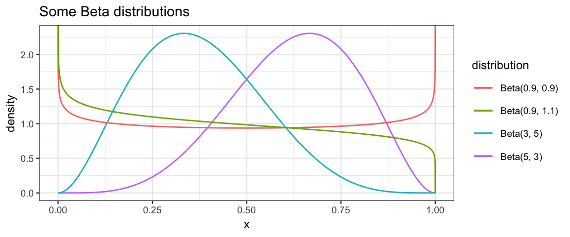

6.2 Beta and Bayes

Suppose we want to estimate a proportion \(\theta\) by repeating some random process (like a coin toss) \(N\) times. We will code each result using a 0 (failure) or a 1 (success): \(Y_1, Y_2, \dots, Y_N\). Here’s our model.
The prior, to be determined shortly, is indicated as ??? for the moment. \[\begin{align*} Y_i & \sim {\sf Bern}(\theta) \\ \theta & \sim{} ??? \end{align*}\]

6.2.1 The Bernoulli likelihood function

The first line turns into the following likelihood function – the probability of observing \(y_i\) for a give parameter value \(\theta\):

\[\begin{align*} Pr{Pr}(Y_i = y_i \mid \theta) = p(y_i \mid \theta) &= \begin{cases} \theta & y_i = 1 \\ (1-\theta) & y_i = 0 \end{cases} \\ &= \theta^{y_i} (1-\theta)^{y_i} \end{align*}\]

The likelihood for the entire data set is then \[\begin{align*} p(\langle y_1, y_2, \dots, y_N \rangle \mid \theta) &= \prod_{i = 1}^N \theta^{y_i} (1-\theta)^{y_i} \\ &= \theta^{x} (1-\theta)^{N - x} \end{align*}\] where \(x\) is the number of “successes” and \(N\) is the number of trials. Since the likelihood only depends on \(x\) and \(N\), not the particular order in which the 0’s and 1’s are observed, we will write the likelihood as

\[\begin{align*} p(x, N \mid \theta) &= \theta^{x} (1-\theta)^{N - x} \end{align*}\]

Reminder: If we think of this expression as a function of \(\theta\) for fixed data (rather than as a function of the data for fixed \(\theta\)), we see that it is the kernel of a \({\sf Beta}(x + 1, N - x + 1)\) distribution. But even thought of this way, the likelihood need not be a PDF – the total sum or integral need not be 1. But we will sometimes normalize likelihood functions if we want to display them on plots with priors and posteriors.

6.2.2 A convenient prior

Now let think about our posterior:

\[\begin{align*} p(\theta \mid x, N) & = \overbrace{p(x, N \mid \theta)}^{\mathrm{likelihood}} \cdot \overbrace{p(\theta)}^{\mathrm{prior}} / p(x, N) \\ & = {\theta^x (1-\theta)^{N - x}} \cdot {p(\theta)} / p(x, N) \end{align*}\] If we let \(p(\theta) = \theta^a (1-\theta^b)\), the product is epsecially easy to evaluate: \[\begin{align*} p(\theta \mid x, N) & = \overbrace{p(x, N \mid \theta)}^{\mathrm{likelihood}} \cdot \overbrace{p(\theta)}^{\mathrm{prior}} / p(x, N) \\ & = {\theta^x (1-\theta)^{N - x}} \cdot {\theta^a (1-\theta)^b)} / p(x, N) \\ & = {\theta^{x+a} (1-\theta)^{N - x + b}} / p(x, N) \end{align*}\] In this happy situation, when mutlipying the likelihood and the prior leads to a posterior with same form as the prior, we say that the prior is a conjugate prior (for that particular likelihood function). So beta priors are conjugate priors for the Bernoulli likelihood, and if we use a beta prior, we will get a beta posterior and it is easy to calculate which one:

prior	data	posterior
\(\sf{Beta}(a, b)\)	\(x, N\)	\({\sf Beta}(x + a, N - x + b)\)

6.2.3 Pros and Cons of conjugate priors

Pros: Easy and fast calculation; can reason about the relationship between prior, likelihood, and posterior based on a known distributions.

Cons: We are restricted to using a conjugate prior, and that isn’t always the prior we want; many situations don’t have natural conjugate priors available; the computations are often not as simple as in our current example.

6.3 Getting to know the Beta distributions

6.3.1 Important facts

You can often look up this sort of information on the Wikipedia page for a family of distributions. If you go to https://en.wikipedia.org/wiki/Beta_distribution you will find, among other things, the following:


Notation	Beta(\(\alpha, \beta\))
Parameters	\(\alpha > 0\) shape (real) \(\beta > 0\) shape (real)
Support	\(\displaystyle x\in [0,1]\) or \(\displaystyle x\in (0,1)\)
PDF	\(\displaystyle \frac{x^{\alpha -1}(1-x)^{\beta -1}}{\mathrm{B}(\alpha, \beta )}\)
Mean	\(\displaystyle \frac{\alpha }{\alpha +\beta }\)
Mode	\(\displaystyle {\frac{\alpha -1}{\alpha +\beta -2}}\) for \(\alpha, \beta > 1\) 0 for \(\alpha = 1, \beta > 1\) 1 for \(\alpha > 1, \beta = 1\)
Variance	\(\displaystyle \frac{\alpha \beta}{(\alpha +\beta )^{2}(\alpha +\beta +1)}\)
Concentration	\(\displaystyle \kappa =\alpha +\beta\)

6.3.2 Alternative parameterizations of Beta distributions

There are several different parameterizations of the beta distributions that can be helpful in selecting a prior or interpreting a posterior.

6.3.2.1 Mode and concentration

Let the concentration be defined as \(\kappa =\alpha +\beta\). Since the mode (\(\omega\)) is \(\displaystyle {\frac{\alpha -1}{\alpha +\beta -2}}\) for \(\alpha, \beta > 1\), we can solve for \(\alpha\) and \(\beta\) to get

\[\begin{align} \alpha &= \omega (\kappa - 2) + 1\\ \beta &= (1-\omega)(\kappa -2) + 1 \end{align}\]

6.3.2.2 Mean and concentration

The beta distribution may also be reparameterized in terms of its mean \(\mu\) and the concentration \(\kappa\). If we solve for \(\alpha\) and \(\beta\), we get

\[\begin{align} \alpha &= \mu \kappa \\ \beta &= (1 - \mu) \kappa \end{align}\]

6.3.2.3 Mean and variance (or standard deviation)

We can also parameterize with the mean \(\mu\) and variance \(\sigma^2\). Solving the system of equations for mean and variance given in the table above, we get

\[\begin{align} \kappa &=\alpha +\beta = \frac{\mu (1-\mu )}{\sigma^2} - 1 \\ \alpha &=\mu \kappa = \mu \left({\frac{\mu (1-\mu )}{\sigma^2}}-1\right) \\ \beta &= (1-\mu )\kappa = (1-\mu ) \left({\frac{\mu (1-\mu)} {\sigma^2}} -1 \right), \end{align}\] provided \(\sigma^2 < \mu (1-\mu)\).

6.3.3 beta_params()

CalvinBayes::beta_params() will compute several summaries of a beta distribution given any of these 2-parameter summaries. This can be very handy for converting from one type of information about a beta distribution to another.

For example. Suppose you want a beta distribution with mean 0.3 and standard deviation 0.1. Which beta distribution is it?

library(CalvinBayes)
beta_params(mean = 0.3, sd = 0.1)

shape1	shape2	mean	mode	sd	concentration
6	14	0.3	0.2778	0.1	20

We can do a similar thing with other combinations.

bind_rows(
  beta_params(mean = 0.3, concentration = 10),
  beta_params(mode = 0.3, concentration = 10),
  beta_params(mean = 0.3, sd = 0.2),
  beta_params(shape1 = 5, shape2 = 10),
)

shape1	shape2	mean	mode	sd	concentration
3.000	7.000	0.3000	0.2500	0.1382	10.00
3.400	6.600	0.3400	0.3000	0.1428	10.00
1.275	2.975	0.3000	0.1222	0.2000	4.25
5.000	10.000	0.3333	0.3077	0.1179	15.00

6.3.4 Automating Bayesian updates for a proportion (beta prior)

Since we have formulas for this case, we can write a function handle any beta prior and any data set very simply. (Much simpler than doing the grid method each time).

quick_bern_beta <- 
  function(
    x, n,     # data, successes and trials
    ...       # see clever trick below
  ) 
  {
    pars <- beta_params(...)
    a <- pars$shape1
    b <- pars$shape2
    
    theta_hat <- x / n  # value that makes likelihood largest
    posterior_mode <- (a + x - 1) / (a + b + n - 2)  
    
    # scale likelihood to be as tall as the posterior
    likelihood <- function(theta) {
      dbinom(x, n, theta) / dbinom(x, n, theta_hat) *
        dbeta(posterior_mode, a + x, b + n - x)  # posterior height at mode
    }
    
    gf_dist("beta", shape1 = a, shape2 = b, 
            color = ~ "prior", alpha = 0.5, xlim = c(0,1), size = 1.2) %>%
      gf_function(likelihood, 
                  color = ~ "likelihood", alpha = 0.5, size = 1.2) %>%
      gf_dist("beta", shape1 = a + x, shape2 = b + n - x, 
              color = ~ "posterior", alpha = 0.5, size = 1.6) %>%
      gf_labs(
        color = "function",
        title = paste0("posterior: Beta(", a + x, ", ", b + n - x, ")")
      ) %>% 
      gf_refine(
        scale_color_manual(
          values = c("prior" = "gray50", "likelihood" = "forestgreen", 
                     "posterior" = "steelblue")))
  }

With such a function in hand, we can explore examples very quickly. Here are three examples from DBDA2e (pp. 134-135).

quick_bern_beta(17, 20, mode = 0.5, k = 500)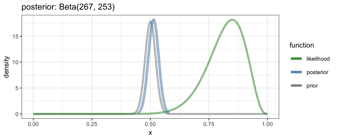

quick_bern_beta(17, 20, mode = 0.75, k = 25)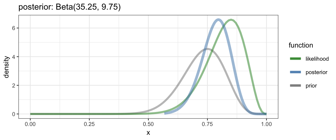

quick_bern_beta(17, 20, a = 1, b = 1)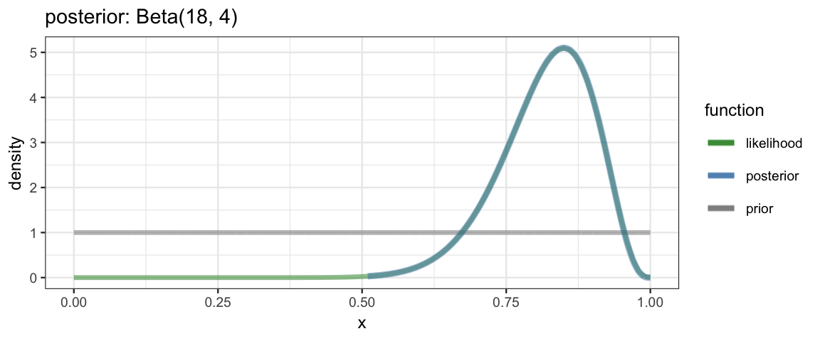

6.4 What if the prior isn’t a beta distribution?

Unless it is some other distribution where we can work things out mathematically, we are back to the grid method.

Here’s an example like the one on page 136.

dtwopeaks <- function(x) {
  0.48 * triangle::dtriangle(x, 0.2, 0.3) +
  0.48 * triangle::dtriangle(x, 0.7, 0.8) +
  0.04 * dunif(x)
}

BernGrid(data = c(rep(0, 13), rep(1, 14)), prior = dtwopeaks) %>%
  gf_function(function(theta) 0.3 * dbinom(13, 27, theta), color = "forestgreen")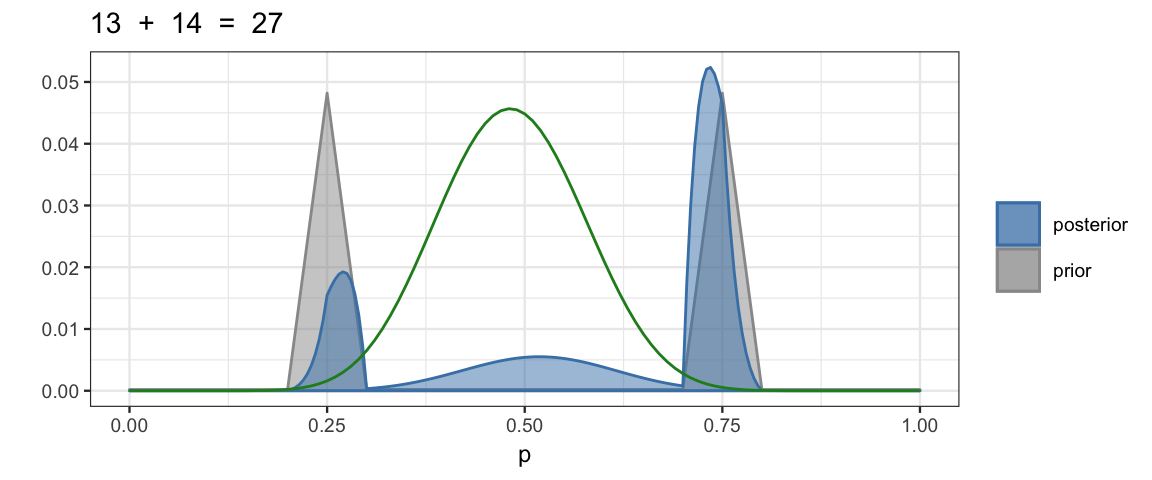

6.5 Exercises

Show that if \(\alpha, \beta > 1\), then the mode of a Beta(\(\alpha\), \(\beta\)) distribution is \(\displaystyle {\frac{\alpha -1}{\alpha +\beta -2}}\).

Hint: What would you do if you were in Calculus I?

Suppose we have a coin that we know comes from a magic-trick store, and therefore we believe that the coin is strongly biased either usually to come up heads or usually to come up tails, but we don’t know which.
1. Express this belief as a beta prior. That is, find shape parameters that lead to a beta distribution that corresponds to this belief.
2. Now we flip the coin 5 times and it comes up heads in 4 of the 5 flips. What is the posterior distribution?
3. Use quick_bern_beta() or a similar function of your own creation to show the prior and posterior graphically.
Suppose we estimate a proprtion \(\theta\) using a \({\sf Beta}(10, 10)\) prior and a observe 26 successes and 48 failures.
1. What is the posterior distribution?
2. What is the mean of the posterior distribution?
3. What is the mode of the posterior distribution?
4. Compute a 90% HDI for \(\theta\). [Hint: qbeta()]
Suppose a state-wide election is approaching, and you are interested in knowing whether the general population prefers the democrat or the republican. There is a just-published poll in the newspaper, which states that of 100 randomly sampled people, 58 preferred the republican and the remainder preferred the democrat.
1. Suppose that before the newspaper poll, your prior belief was a uniform distribution. What is the 95% HDI on your beliefs after learning of the newspaper poll results?
2. Based on what you know about elections, why is a uniform prior not a great choice? Repeat part (a) with a prior the conforms better to what you know about elections. How much does the change of prior affect the 95% HDI?
3. You find another poll conducted by a different news organization In this second poll, 56 of 100 people preferred the republican. Assuming that peoples’ opinions have not changed between polls, what is the 95% HDI on the posterior taking both polls into account. Make it clear which prior you are using.
4. Based on this data (and your choice of prior, and assuming public opinion doesn’t change between the time of the polls and election day), what is the probability that the republican will win the election.