19 Nominal Predictors

19.1 Fruit flies Study

A study of fruit flies (Hanley & Shapiro, 1994) considered whether the female companions (none, 1 pregnant, 8 pregnant, 1 virgin, or 8 virgin) is associated with differences in longevity of males (measured in days).

gf_violin(longevity ~ group, data = FruitflyReduced) %>%
  gf_jitter(width = 0.2, height = 0, alpha = 0.5) %>%
  gf_point(stat = "summary", color = "red", size = 3, alpha = 0.5, fun = mean)

## No summary function supplied, defaulting to `mean_se()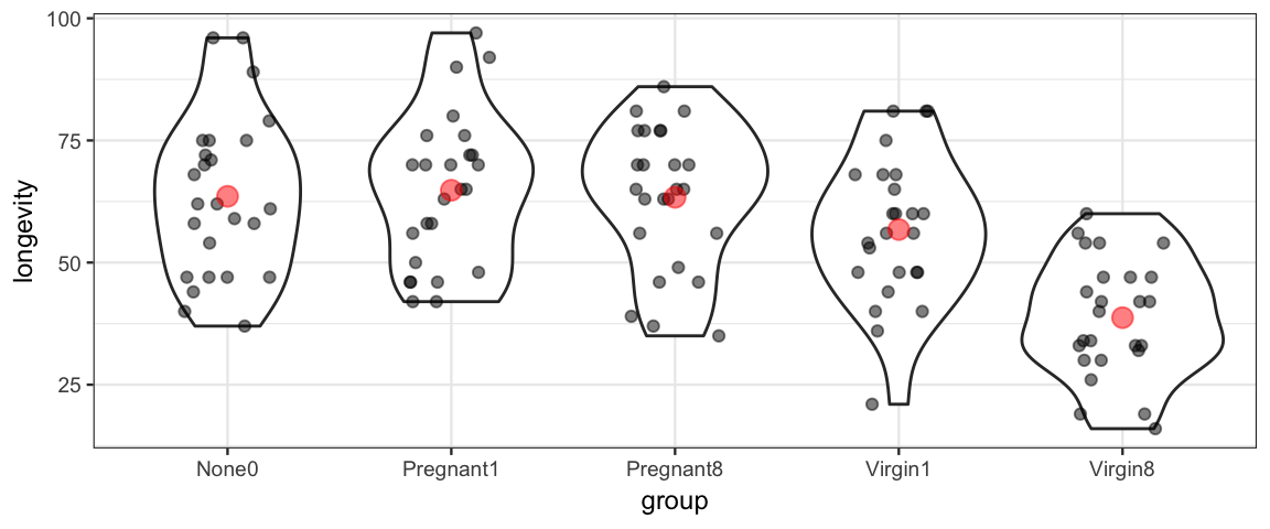

19.2 Model 1: Out-of-the-box

It is easy enough to ask brm() to fit a model for us. Let’s just give it our explanatory and response variables and see what happens.

flies_brm <- brm(longevity ~ group, data = FruitflyReduced)

## Compiling the C++ model

## Start sampling

flies_stan <- stanfit(flies_brm)
flies_stan

## Inference for Stan model: 2838b68e72ce876b17fbd0e486bccf49.
## 4 chains, each with iter=2000; warmup=1000; thin=1; 
## post-warmup draws per chain=1000, total post-warmup draws=4000.
## 
##                     mean se_mean   sd    2.5%     25%     50%     75%   97.5% n_eff Rhat
## b_Intercept        63.48    0.06 3.00   57.73   61.39   63.54   65.52   69.24  2711    1
## b_groupPregnant1    1.46    0.07 4.20   -6.58   -1.27    1.39    4.25    9.77  3259    1
## b_groupPregnant8   -0.09    0.08 4.30   -8.65   -2.95   -0.06    2.81    8.21  3018    1
## b_groupVirgin1     -6.72    0.07 4.24  -14.90   -9.59   -6.73   -3.91    1.70  3278    1
## b_groupVirgin8    -24.71    0.08 4.21  -32.86  -27.54  -24.69  -21.79  -16.52  3059    1
## sigma              14.92    0.02 0.95   13.20   14.26   14.85   15.53   16.92  3996    1
## lp__             -519.59    0.04 1.73 -523.63 -520.54 -519.29 -518.30 -517.10  1711    1
## 
## Samples were drawn using NUTS(diag_e) at Wed May  1 22:34:15 2019.
## For each parameter, n_eff is a crude measure of effective sample size,
## and Rhat is the potential scale reduction factor on split chains (at 
## convergence, Rhat=1).

mcmc_combo(as.mcmc.list(flies_stan))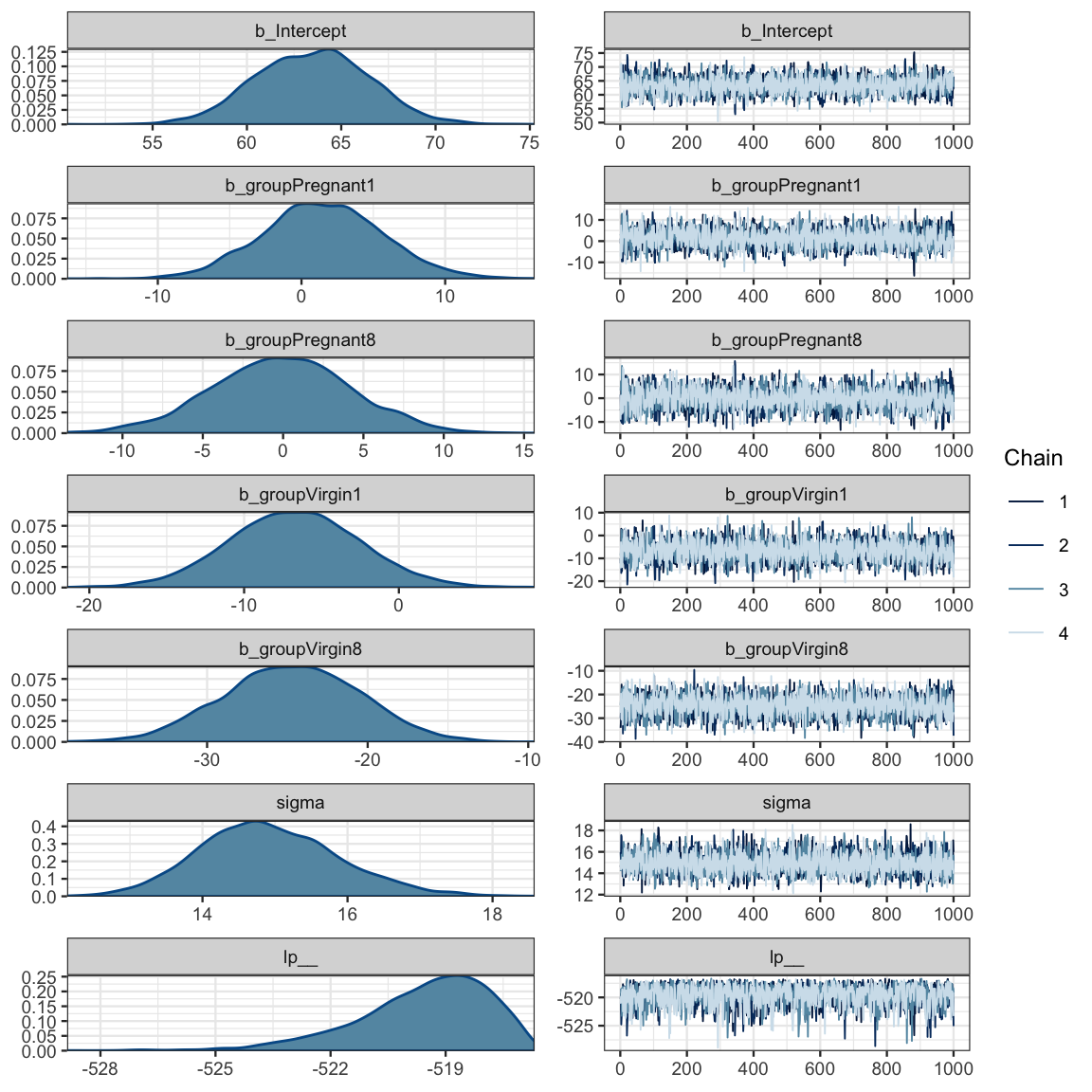

mcmc_areas_ridges(as.mcmc.list(flies_stan), regex_pars = "b_g")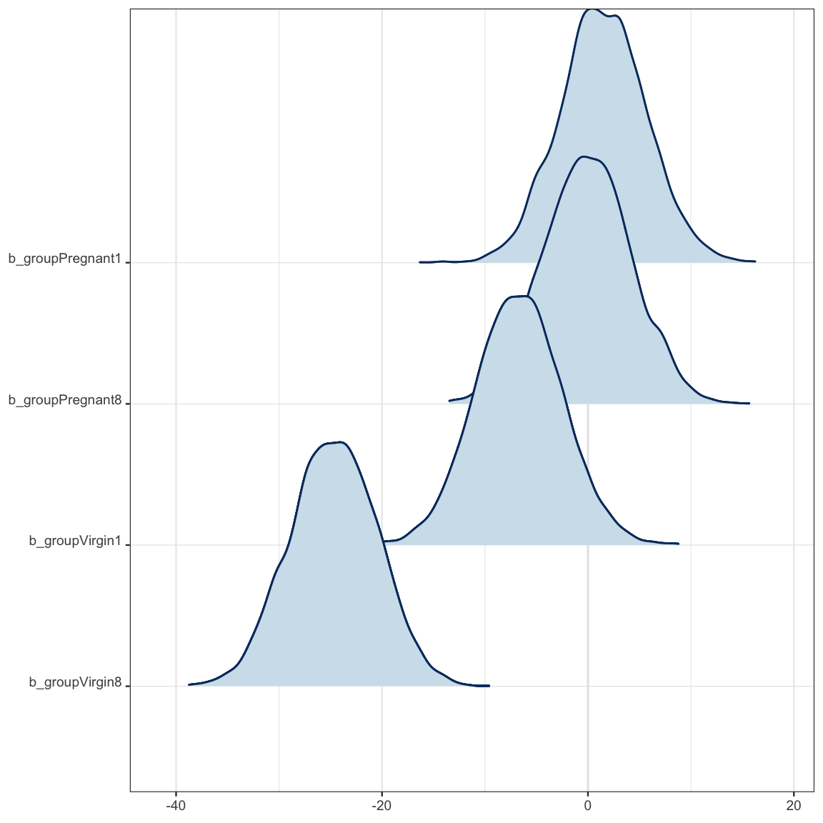

But what just happened? Why do we have 5 parameters starting with b_? Our first clue comes from looking at the data that get sent to Stan.

standata(flies_brm) %>% lapply(head)

## $N
## [1] 125
## 
## $Y
## [1] 35 37 49 46 63 39
## 
## $K
## [1] 5
## 
## $X
##   Intercept groupPregnant1 groupPregnant8 groupVirgin1 groupVirgin8
## 1         1              0              1            0            0
## 2         1              0              1            0            0
## 3         1              0              1            0            0
## 4         1              0              1            0            0
## 5         1              0              1            0            0
## 6         1              0              1            0            0
## 
## $prior_only
## [1] 0

Our group variable has been turned into 4 (really 5, if you count the intercept, which is all 1’s) new 0/1 variables. So our model is

\[\begin{align*} \mathrm{longevity} &= \beta_0 \cdot 1 + \beta_1 x_1 + \beta_2 x_2 + \beta_3 x_3 + \beta_4 x_4 + \mathrm{noise} \\ & = \beta_0 \cdot 1 + \beta_1 x_1 + \beta_2 x_2 + \beta_3 x_3 + \beta_4 x_4 + {\sf Norm}(0, \sigma) \end{align*}\]

where, for example,

\[\begin{align*} x_1 &= [\![ \mbox{group} = \mbox{Pregnant1} ]\!] \\ &= \begin{cases} 1 & \mbox{if group} = \mbox{Pregnant1} \\ 0 & \mbox{if group} \neq \mbox{Pregnant1} \end{cases} \end{align*}\]

In other words the distribution of longevity is

\({\sf Norm}(\beta_0, \sigma)\) for the None0 group
\({\sf Norm}(\beta_0 + \beta_1, \sigma)\) for the Pregnant1 group
\({\sf Norm}(\beta_0 + \beta_2, \sigma)\) for the Pregnant2 group
\({\sf Norm}(\beta_0 + \beta_3, \sigma)\) for the Virgin1 group
\({\sf Norm}(\beta_0 + \beta_4, \sigma)\) for the Virgin2 group

Here are the default priors.

prior_summary(flies_brm)

prior	class	coef
	b
	b	groupPregnant1
	b	groupPregnant8
	b	groupVirgin1
	b	groupVirgin8
student_t(3, 58, 18)	Intercept
student_t(3, 0, 18)	sigma

Flat improper priors for the b_ parameters.
t-distribution with 3 degrees of freedom for the intercept (heavier tails than a normal distribution)
- Note: This is really a prior for \(\alpha_0\), not \(\beta_0\) since it is usually easier to specify a prior for \(\alpha_0\). If for some reason we wanted to specify a prior for \(\beta_0\) instead, there is a little trick: use the formula longevity ~ 0 + intercept + group.
- If you are curious where 58 and 18 came from, here’s a good guess:
```
df_stats(~ longevity, data = FruitflyReduced, mean, sd)
```
mean_longevity sd_longevity

57.44 17.56

That is, the prior says that the mean response at the mean value of the predictor (in the data) should be roughly the mean value of the responsss in the data, and our uncertainty is on the scale of the variability in responses in the data.
“T” for sigma. (This is really a “half t”, since Stan knows the parameter must be positive.)

mean_longevity	sd_longevity
57.44	17.56

19.3 Model 2: Custom Priors

The out-of-the-box model above differs from the basic model in DBDA.

We can get closer to the DBDA model using this:

flies2_brm <- 
  brm(longevity ~ group, data = FruitflyReduced,
      prior = c(
        set_prior(class = "Intercept", "normal(60, 100)"),  # 100 = 5 * 20
        set_prior(class = "b", "normal(0, 10)"),  # group = "b" is default; could be omitted
        set_prior(class = "sigma", "uniform(20.0/1000.0, 20.0 * 1000.0)")
      )
  )

## Compiling the C++ model

## Start sampling

prior_summary(flies2_brm)
stancode(flies2_brm)

This still isn’t exactly the same as the model used by Kruschke. It turns out that there are multiple ways to code the \(\beta\)s. The model we just fit and one more are easy to do with brm(). A third is used by Kruschke and takes a bit more work to fit using brm().

19.4 Models 3 and 4: alternate parameterizations

If we remove the intercept in the brm() model, we get a model with a \(\beta_i\) for each group mean rather than \(\beta_0\) for the first group and \(\beta_i\) for the difference in group means when \(i > 0\):

flies3_brm <- 
  brm(
    longevity ~ 0 + group, data = FruitflyReduced,
    prior = c(
      set_prior(class = "b", "normal(60, 10)"),  # group = "b" is default; could be omitted
      set_prior(class = "sigma", "uniform(20.0/1000.0, 20.0 * 1000.0)")
    ),
    sample_prior = TRUE
  )

## Compiling the C++ model

## Start sampling

prior_summary(flies3_brm)
stancode(flies3_brm)

This is equivalent to

\[\begin{align*} \mathrm{longevity} &= \beta_0 x_0 + \beta_1 x_1 + \beta_2 x_2 + \beta_3 x_3 + \beta_4 x_4 + \mathrm{noise} \\ & = \beta_0 x_0 + \beta_1 x_1 + \beta_2 x_2 + \beta_3 x_3 + \beta_4 x_4 + {\sf Norm}(0, \sigma) \end{align*}\]

where, for example,

\[\begin{align*} x_1 &= [\![ \mbox{group} = \mbox{Pregnant1} ]\!] \\ &= \begin{cases} 1 & \mbox{if group} = \mbox{Pregnant1} \\ 0 & \mbox{if group} \neq \mbox{Pregnant1} \end{cases} \end{align*}\]

In other words the distribution of longevity is

\({\sf Norm}(\beta_0, \sigma)\) for the None0 group
\({\sf Norm}(\beta_1, \sigma)\) for the Pregnant1 group
\({\sf Norm}(\beta_2, \sigma)\) for the Pregnant2 group
\({\sf Norm}(\beta_3, \sigma)\) for the Virgin1 group
\({\sf Norm}(\beta_4, \sigma)\) for the Virgin2 group

Kruschke uses an overspecified model that has 6 parameters: an intercept and 5 “offsets”. An extra step has to be included to properly specify the model. His model is designed so that \(\beta_0\) is an overall average and the other \(\beta_i\)’s give differences to that overall average.

I haven’t figured out if there is an easy way to do this with brm(). But with a little work, we can force it. The key to doing this is the use of stanvar() to create additional lines of code that are injected into the Stan code. We use scode to give the desired code (as a string) and block to say which Stan block to put it in.

FruitflyReduced <-
  FruitflyReduced %>% mutate(one = 1)
flies4_brm <- 
  brm(
    longevity ~ 0 + one + group, data = FruitflyReduced,
    prior = c(
      set_prior(coef = "one", "normal(60,10)"),
      set_prior(class = "b", "normal(0, 10)"),  # group = "b" is default; could be omitted
      set_prior(class = "sigma", "uniform(20.0/1000.0, 20.0 * 1000.0)")
    ),
    sample_prior = TRUE,
    stanvars = 
      c(
        # compute the average average
        stanvar(scode = "  real a_one = mean(b[2:K]) + b[1];", block = "genquant"),
        # compute the offsets to the average average
        stanvar(scode = "  vector[K - 1] a = b[1] + b[2:K] - a_one;", block = "genquant")
      )
  )

## Compiling the C++ model

## Start sampling

prior_summary(flies4_brm)
stancode(flies4_brm)

mcmc_areas(as.mcmc.list(stanfit(flies4_brm)), regex_pars = c("a_one", "a\\[", "^b_"))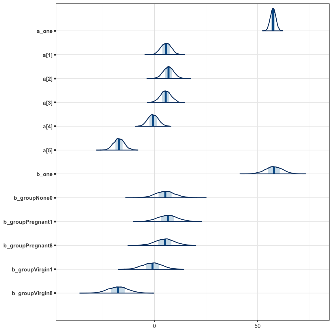

As we can see, the modes of the posteriors for the a and b parameters are similar (because the prior on b_one kept b_one from drifting too far from where a_one is centered), but the posteriors for the a parameters are significantly narrower, so the conversion from b’s to a’s is important.

19.5 Comparing groups

19.5.1 Comparing to the “intercept group”

Let’s return to model 2.

stanfit(flies2_brm)

## Inference for Stan model: bf639a104df81234b81629296b75e83c.
## 4 chains, each with iter=2000; warmup=1000; thin=1; 
## post-warmup draws per chain=1000, total post-warmup draws=4000.
## 
##                     mean se_mean   sd    2.5%     25%     50%     75%   97.5% n_eff Rhat
## b_Intercept        61.68    0.05 2.63   56.43   59.92   61.73   63.50   66.60  3156    1
## b_groupPregnant1    2.87    0.06 3.79   -4.29    0.34    2.77    5.40   10.54  3613    1
## b_groupPregnant8    1.57    0.06 3.83   -5.87   -0.95    1.54    4.19    9.17  3713    1
## b_groupVirgin1     -4.46    0.06 3.84  -11.81   -7.05   -4.53   -1.93    3.24  3657    1
## b_groupVirgin8    -21.10    0.06 3.79  -28.37  -23.70  -21.09  -18.56  -13.59  3683    1
## sigma              14.97    0.01 0.98   13.19   14.29   14.92   15.58   17.07  4315    1
## lp__             -543.27    0.04 1.78 -547.62 -544.18 -542.92 -541.98 -540.81  1770    1
## 
## Samples were drawn using NUTS(diag_e) at Wed May  1 22:35:06 2019.
## For each parameter, n_eff is a crude measure of effective sample size,
## and Rhat is the potential scale reduction factor on split chains (at 
## convergence, Rhat=1).

In this model, one group corresponds to the intercept of the model, and comparisons of other groups to this group is a matter of investigating the posterior distribution of one of the other \(\beta\)’s.

flies_post <- posterior(flies_stan)
names(flies_post)

## [1] "b_Intercept"      "b_groupPregnant1" "b_groupPregnant8" "b_groupVirgin1"   "b_groupVirgin8"  
## [6] "sigma"            "lp__"             "chain"            "iter"

plot_post(flies_post$b_groupPregnant1)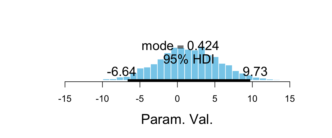

## $posterior
##       ESS mean median   mode
## var1 3226 1.46  1.395 0.4242
## 
## $hdi
##   prob     lo    hi
## 1 0.95 -6.641 9.727

hdi(flies_post$b_groupPregnant1)

par	lo	hi	mode	prob
var1	-6.641	9.727	2.438	0.95

plot_post(flies_post$b_groupVirgin1)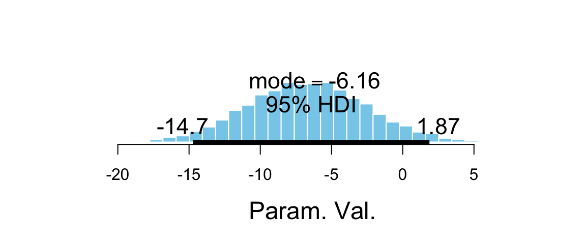

## $posterior
##       ESS   mean median   mode
## var1 3173 -6.719 -6.728 -6.163
## 
## $hdi
##   prob     lo    hi
## 1 0.95 -14.72 1.874

mcmc_areas(as.mcmc.list(flies_stan), pars = "b_groupVirgin1", prob = 0.95)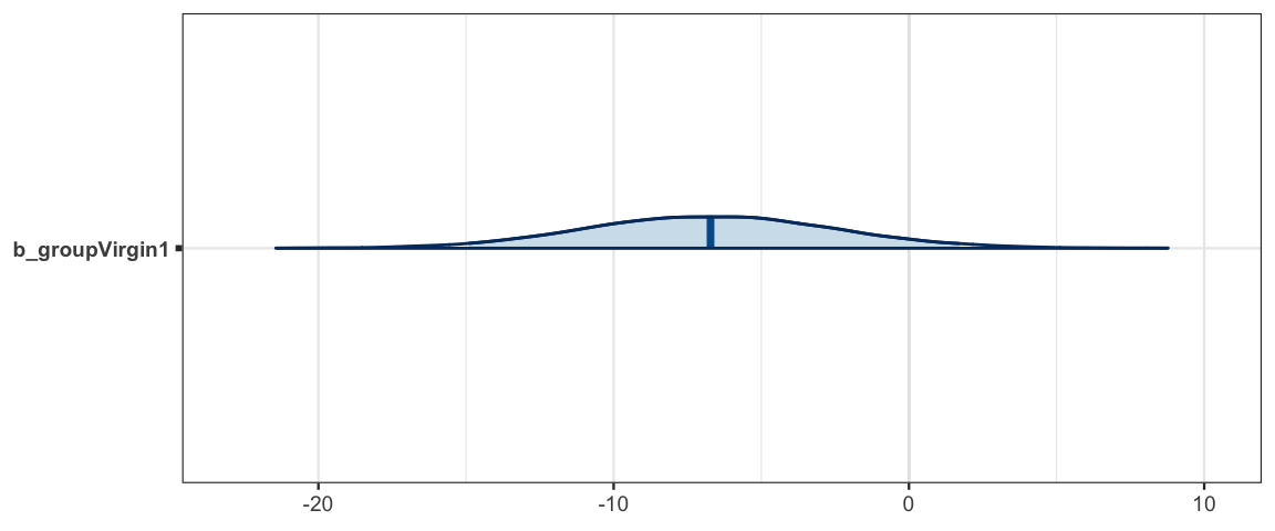

hdi(flies_post$b_groupVirgin1)

par	lo	hi	mode	prob
var1	-14.72	1.874	-6.802	0.95

19.5.2 Comparing others pairs of groups

What if we want to compare the Virgin1 and Virgin8 groups? We can use the identity \(\beta_0 + \beta_i - (\beta_0 + \beta_j) = \beta_i - \beta_j\) to simplify the algebra and do it this way. (The same would work in model 3 or 4 as well.)

flies_post <-
  flies_post %>% mutate(dVirgin = b_groupVirgin8 - b_groupVirgin1)
plot_post(flies_post$dVirgin, xlab = "Virgin8 - Virgin1")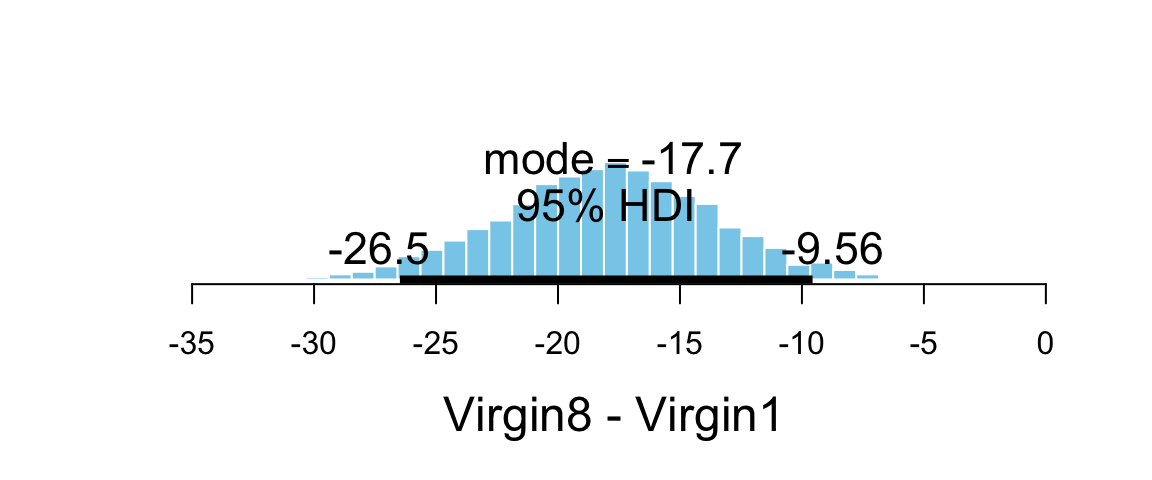

## $posterior
##       ESS   mean median   mode
## var1 6589 -17.99 -17.94 -17.73
## 
## $hdi
##   prob     lo     hi
## 1 0.95 -26.48 -9.564

19.5.3 Contrasts: Comparing “groups of groups”

What if we want to compare the two virgin groups to the 3 other groups? This is a bit simpler to do using the model without an intercept term.

flies3_post <- posterior(flies3_brm)
names(flies3_post)

## [1] "b_groupNone0"     "b_groupPregnant1" "b_groupPregnant8" "b_groupVirgin1"   "b_groupVirgin8"  
## [6] "sigma"            "prior_b"          "prior_sigma"      "lp__"

flies3_post <-
  flies3_post %>% 
  mutate(
    contrast = 
      (b_groupVirgin8 + b_groupVirgin1)/2 - 
      (b_groupPregnant1 + b_groupPregnant8 + b_groupNone0) / 3
)
plot_post(flies3_post$contrast, xlab = "Virgin vs non-virgin groups")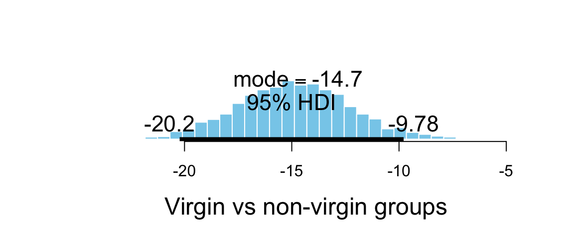

## $posterior
##       ESS   mean median  mode
## var1 5755 -14.87 -14.89 -14.7
## 
## $hdi
##   prob     lo     hi
## 1 0.95 -20.23 -9.784

The expression

\[\begin{align*} \frac{\mu_3 + \mu_4}{2} - \frac{\mu_0 + \mu_1 + \mu_2}{3} &= -\frac13 \mu_0 -\frac13 \mu_1 -\frac13 \mu_2 + \frac12 \mu_3 + \frac12 \mu_4 \end{align*}\]

is an example of a contrast. A contrast is simply a linear combination of the group means such that the sum of the coefficients is 0. Many interesting relationships can be investigated using contrasts, and the brms package includes the hypothesis() function to help us do this. (Note: because we included sample_prior = TRUE in the call to brm() for this model, the plot below shows both prior and posterior distributions for the contrast.)

h <-
  hypothesis(
    flies3_brm,
    "(groupVirgin8 + groupVirgin1) / 2 < 
      (groupPregnant1 + groupPregnant8 + groupNone0) / 3"
  )
h

## Hypothesis Tests for class b:
##                 Hypothesis Estimate Est.Error CI.Lower CI.Upper Evid.Ratio Post.Prob Star
## 1 ((groupVirgin8+gr... < 0   -14.87      2.65     -Inf   -10.43        Inf         1    *
## ---
## '*': The expected value under the hypothesis lies outside the 95%-CI.
## Posterior probabilities of point hypotheses assume equal prior probabilities.

plot(h)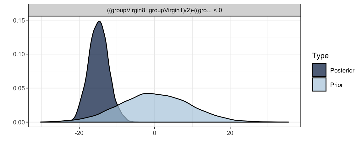

19.5.3.1 Multiple Hypotheses at once

We can even test multiple hypotheses at once.

h2 <-
  hypothesis(
    flies3_brm,
    c("groupVirgin1 < (groupPregnant1 + groupPregnant8 + groupNone0) / 3",
      "groupVirgin8 < (groupPregnant1 + groupPregnant8 + groupNone0) / 3")
  )
h2

## Hypothesis Tests for class b:
##                 Hypothesis Estimate Est.Error CI.Lower CI.Upper Evid.Ratio Post.Prob Star
## 1 (groupVirgin1)-((... < 0    -6.60      3.35     -Inf    -1.09      38.22      0.97    *
## 2 (groupVirgin8)-((... < 0   -23.15      3.38     -Inf   -17.48        Inf      1.00    *
## ---
## '*': The expected value under the hypothesis lies outside the 95%-CI.
## Posterior probabilities of point hypotheses assume equal prior probabilities.

plot(h2)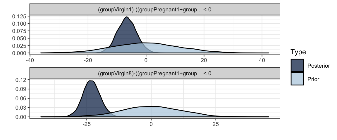

19.5.3.2 Equality or inequality?

In the previous example, we expressed our contrast as an inequality. We can also express it as an equality. The output that we get from hypothesis() is a bit different if we do so.

h3 <-
  hypothesis(
    flies3_brm,
    c("groupVirgin1 = (groupPregnant1 + groupPregnant8 + groupNone0) / 3",
      "groupVirgin8 = (groupPregnant1 + groupPregnant8 + groupNone0) / 3")
  )
h3

## Hypothesis Tests for class b:
##                 Hypothesis Estimate Est.Error CI.Lower CI.Upper Evid.Ratio Post.Prob Star
## 1 (groupVirgin1)-((... = 0    -6.60      3.35   -13.37     0.03       0.53      0.35     
## 2 (groupVirgin8)-((... = 0   -23.15      3.38   -29.77   -16.34       0.00      0.00    *
## ---
## '*': The expected value under the hypothesis lies outside the 95%-CI.
## Posterior probabilities of point hypotheses assume equal prior probabilities.

plot(h3)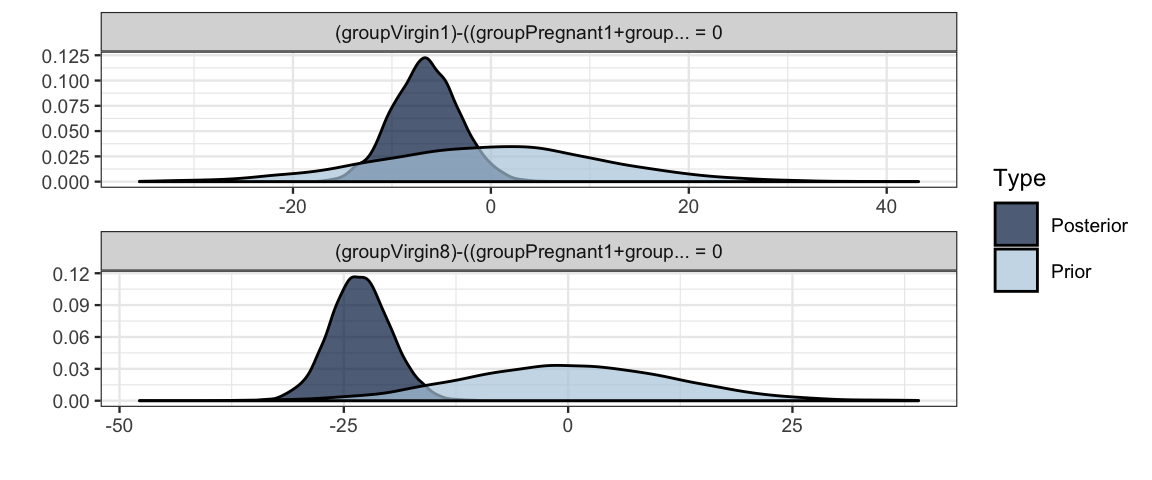

The CI is 2-sided rather than 1-sided.
Evidence Ratio is defined differently.
- For inequalities, this is the ratio of the posterior probabilities for the inequality being true vs. false
- For equalities, this is the ratio of the posterior density (of the equality holding) to the prior density. (This only works if sample_prior = TRUE since prior samples are required to make the calculation.)

19.6 More Variations

The models we have looked at above are very similar to a traditional ANOVA model, the key features of which are

normal distributions for each group (normal noise), and
same standard deviation in each group (homoskedasticity).

In frequentist statistics, these are largely chosen for convenience (the mathematics is much easier). But we can easily relax these restrictions using Bayesian software. Let’s fit a model using

t distributions instead normal distributions for the noise.

This will make the results more robust against outliers in our sample or distributions with heavier tails.
different standard deviation parameters for each group.

Both are easy to do with brm(). The main new feature is the use of bf() to provide two formulas. The first describes the mean response (separate means for each group). The second formula describes sigma (separate values for each group). The rest should look familiar.

flies5_brm <- 
  brm(
    bf(longevity ~ 0 + group, sigma ~ 0 + group),
    data = FruitflyReduced,
    family = student(),   # t distribution for the noise
    prior = c(
      set_prior(class = "b", "normal(60, 10)")
    ),
    sample_prior = TRUE
  )

## Compiling the C++ model

## Start sampling

The Stan code for this model includes the following model section.

model {
  vector[N] mu = X * b;
  vector[N] sigma = X_sigma * b_sigma;
  for (n in 1:N) {
    sigma[n] = exp(sigma[n]);
  }
  // priors including all constants
  target += normal_lpdf(b | 60, 10);
  target += gamma_lpdf(nu | 2, 0.1)
    - 1 * gamma_lccdf(1 | 2, 0.1);
  // likelihood including all constants
  if (!prior_only) {
    target += student_t_lpdf(Y | nu, mu, sigma);
  }
}

Note that the values of sigma are on the log scale and are converted (via exp()) to the natural scale before using them in the likelihood function. The sort of encoding of groups is used for (log) sigma as was used for the group means. Because we included 0 in our formula, we get a (log) sigma for each group. This is reported in the summary output for the brm model as a log link for sigma.

flies5_brm

##  Family: student 
##   Links: mu = identity; sigma = log; nu = identity 
## Formula: longevity ~ 0 + group 
##          sigma ~ 0 + group
##    Data: FruitflyReduced (Number of observations: 125) 
## Samples: 4 chains, each with iter = 2000; warmup = 1000; thin = 1;
##          total post-warmup samples = 4000
## 
## Population-Level Effects: 
##                      Estimate Est.Error l-95% CI u-95% CI Eff.Sample Rhat
## groupNone0              63.00      3.22    56.81    69.40       6962 1.00
## groupPregnant1          64.12      3.18    57.75    70.19       6857 1.00
## groupPregnant8          63.37      2.96    57.49    69.11       7327 1.00
## groupVirgin1            57.17      2.90    51.41    62.85       7191 1.00
## groupVirgin8            40.03      2.45    35.30    44.94       6739 1.00
## sigma_groupNone0         2.78      0.16     2.50     3.10       7931 1.00
## sigma_groupPregnant1     2.73      0.16     2.44     3.06       7940 1.00
## sigma_groupPregnant8     2.66      0.15     2.39     2.98       6746 1.00
## sigma_groupVirgin1       2.68      0.16     2.39     3.00       8859 1.00
## sigma_groupVirgin8       2.49      0.15     2.20     2.81       7824 1.00
## 
## Family Specific Parameters: 
##    Estimate Est.Error l-95% CI u-95% CI Eff.Sample Rhat
## nu    27.47     14.96     7.92    65.65       6412 1.00
## 
## Samples were drawn using sampling(NUTS). For each parameter, Eff.Sample 
## is a crude measure of effective sample size, and Rhat is the potential 
## scale reduction factor on split chains (at convergence, Rhat = 1).

mcmc_areas_ridges(as.mcmc.list(stanfit(flies5_brm)), regex_pars = "sigma")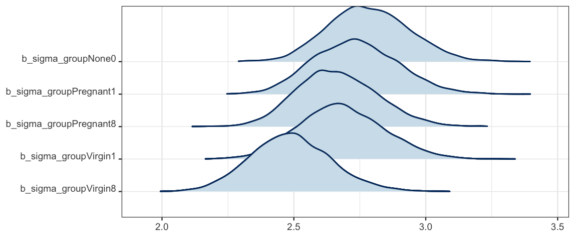

In this case, it doesn’t appear that there is a large difference among the (log) standard deviations in the five groups, but it is noteable that the group with the lowest longevity also has the smallest standard deviation. It is not uncommon for variability to larger when values are larger. Fortunately, it is no harder to fit a model with separate standard deviations than with one standard deviation for all of the groups. And if there substantial differences in the standard deviations, a model that takes that into account will perform better.

If we prefer to see the standard deviations on the natural scale, we can tell Stan to compute and store those values. The naming isn’t quite as nice, however.

flies5a_brm <- 
  brm(
    bf(longevity ~ 0 + group, sigma ~ 0 + group),
    data = FruitflyReduced,
    family = student(),   # t distribution for the noise
    prior = c(
      set_prior(class = "b", "normal(60, 10)")
    ),
    sample_prior = TRUE,
    stanvars = 
      stanvar(
        scode = "vector[K_sigma] b_rsigma = exp(b_sigma);",
        block = "genquant")
  )

## Compiling the C++ model

## Start sampling

flies5a_stan <- stanfit(flies5a_brm)
mcmc_areas_ridges(as.mcmc.list(flies5a_stan), regex_pars = "rsigma")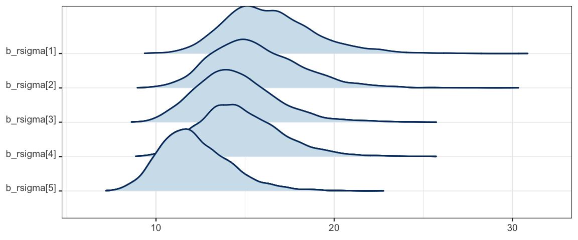

hdi(posterior(flies5a_stan), regex_pars = "rsigma")

par	lo	hi	mode	prob
b_rsigma.1	11.787	21.52	15.68	0.95
b_rsigma.2	11.005	20.49	15.84	0.95
b_rsigma.3	10.398	19.07	14.93	0.95
b_rsigma.4	10.892	19.54	14.27	0.95
b_rsigma.5	8.527	16.12	11.58	0.95

19.7 Exercises

It turns out that larger fruit flies tend to live longer. we can take this into account by adding thorax (the length of each fruit fly’s thorax in mm) to our model. Since we are primarily interested in the association between group and longevity, thorax is referred to as a covariate. But if we were primarily interested in the relationship between longevity and size, we could use the same model and call group the covariate. Same model, different focus.

Fit two models: Let Model 1 be the model below and let Model 2 be one just like it but without thorax. Then answer the questions that follow. We’ll stick with the default priors for now, but it would be easy enough to choose your own.
```
model1_brm <-
  brm(
    bf(longevity ~ group + thorax, sigma ~ group + thorax),
    data = FruitflyReduced, 
    family = student(),
  )
```
1. Does Model 1 think that longevity is different for large and small fruit flies? How do you know? How can you quantify your answer?
2. We are primarily interested in whether the fruit flies that live with virgin females live less long than the others (those that live alone or with pregnant females). Using each model, compute a 95% HDI for the contrast that measures this. For Model 1, does it matter what value thorax has? (If yes, use thorax = 0.8 as an example.) How do the two HDI’s compare? Why?
3. Using each model, compute a 95% HDI for the contrast that compares just the Virgin1 flies to the three types of controls (None0, Pregnant1, and Pregnant8). How do the two models compare?
4. Now compare the values for sigma in the two models. To do this, we will need to specify both the group and the thorax size (since for different combinations of these the models estimate different values of sigma). For each of the combinations below, compute a 95% HDI for sigma in two models, one with thorax and one without. Don’t forget to convert to the natural scale. (Recall that brm() uses a log link for sigma.)
  1. group: Pregnant1; thorax: 0.7mm, 0.8mm, 0.9mm [That’s three different HDI’s for Model 1 and the same HDI 3 times for Model 2.]
  2. group: Virgin8; thorax: 0.7mm, 0.8mm, 0.9mm
  How do the results compare for the two models?
5. Given the results above, is it important to include thorax in the model? Explain.
6. Bonus (optional): Create a plot that shows the HDIs for sigma for every combination of model, group, and thorax measurement of 0.6, 0.7, 0.8, or 0.9 mm.