7 D3

7.1 Getting Set Up for D3

7.1.1 Downloading D3

You can use D3 in your websites by referencing an appropriate URL in the head of your HTML document:

<script src="https://d3js.org/d3.v5.min.js"></script>

But it can be useful to have a local copy as well. You can find a link to download the most recent version at https://d3js.org/.

7.1.2 Running a server

To view our web pages we need some sort of server running. We have several options, and different options make sense at different points in the development process.

7.1.2.1 Servers in Editors

Some editors (like Atom and VS Code) have built-in servers to render the files you are editing. In VS Code, install the Live Sever extension. You can launch a live server by searching for it in the command palette:

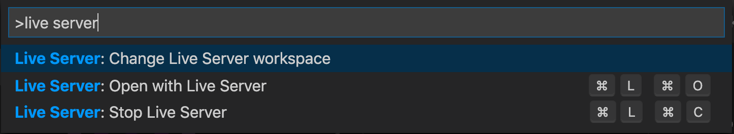
Alternatively, you can right click on your HTML file and select “Open with Live Server”.

Either way, a web page will open with your HTML page rendered. Each time you save, the browser will refresh automatically.

7.1.2.2 Python Simple Server

This is a simple web server written in python.

python -m SimpleHTTPServer

7.1.2.3 Node’s hot-server

This server will auto refresh when you document changes. This can be nice since you can watch things refresh in the browser without having to click or refresh anything. But the JavaScript state is not completely restarted, so sometimes this leads to unusual behavior that would not happen if the page were refreshed.

hot-server

Note: If you want to install this on your own machine, start by installing node and npm.

7.1.2.4 GitHub pages

GitHub pages. GitHub can be configured to serve pages in the /docs folder of your master branch. This is a good way to make pages available to others.

7.1.3 D3 in the browser console

Here’s a little code you can copy and paste into the browser console to enable the use of D3, even if the web page didn’t originally use D3.

// from https://gist.github.com/dwtkns/7568721
var s  = document.createElement('script'); 
s.type = 'text/javascript'; 
s.src  = 'https://d3js.org/d3.v5.min.js'; 
document.head.appendChild(s);

This is roughly equivalent to inserting

<script type = "text/javascript" src = `https://d3js.org/d3.v5.min.js">` 

into the head of the document. But note that we are not editing the HTML, only the DOM.

7.1.4 Chrome’s JavaScript Console

[Note: Other browsers have similar features.]

Chrome’s developer tools, including the JavaScript console can be very useful for debugging a web page that uses JavaScript. This is where output logged with console.log() appears, but you can also run JavaScript code here.

1. Open a web page in Chrome and then open the Developer Tools. You should see a tab labeled Console. In this console you can type javascript code and run it. Give it a try.

   1. Try a little arithmetic: Type 1 + 1 and hit enter.

   2. Create two variables called a and b. Assign a to the number 17 and b to the string 'Hello there!'.

   3. Type a + b and hit enter. Why do you get the results you get?

   4. Create a variable c and assign it to an array of at least 3 elements. You may put into the array whatever you like.

   5. Use javascript to display an array that consists of the first two elements of the array c you just created.

   6. Create an array d that contains the numbers 1 to 100.

   7. Create an array e that contains the squares of the numbers from 1 to 100.

7.2 Selections

7.2.1 some examples to get us started

D3 selectors work much like CSS selectors. The two key functions are

• d3.select(): returns a selection containing the first element of the DOM that matches the selector.
• d3.selectAll(): returns a selection containing all elements of the DOM that match the selector.

A selection is a javascript object that behaves much like an array with some additional methods. These methods let us act on the element of the DOM contained in the selection.

Once we have a selection in hand, we can use JavaScript to find out information about the selection or to modify those elements of the DOM that belong to the selection. Let’s give it a try, then we will figure out how it works.

2. See if you can guess what the following code will do. Then run the code in the Console and see if you were correct.

d3.select("body")
  .append("p")
  .text("Here is some new text.")
  .style("color", "red")

3. Now try this one.

d3.selectAll("p")
  .text("Here is some new text.")
  .style("color", "maroon")
  .style("background-color", "gold")

7.2.2 Method chaining one link at a time

Now let’s take a closer look at how the method chaining is working in the first example above.

d3.select("body")

• d3 is the D3 object and is typically where things will get started.

d3.select("body")

• The select() method finds the first body element in the web page and returns a selection containing that element.

  .append("p")

• This appends to end of the selected body (but just inside it – ie, before the closing tag). In this case, we add a new p element. The object returned by this operation is a selection containing this p element. Importantly, it is still a selection, but it is not the same selection as before.

.text("Here is some new text.")

• .text() adds content to the selected p element and again returns a selection containing this (now modified) p element.

  .style("color", "red")

• This adds style (much like we would add in CSS) to the selected elements – in this case that same p element we just inserted text into. In this case we style the color to be red. Once again the returned value is a selection containing this single p element.

As in the example above, many (but not all) selection methods return another selection. This makes the chaining syntax work so well. But it important to know what selection is being returned or when something else is returned because each method must apply to the type of thing returned by the previous method or the chain will break.

The D3 API Reference specifies what type of object is returned from each method. You can access it at one of the following sites:

• https://devdocs.io/d3~5/
• https://github.com/d3/d3/blob/master/API.md

7.2.3 Breaking chains

We don’t have to use method chaining. Here is a similar example without method chaining. (It’s enough different that you will be able to see it working, but the structure is the same.)

let s1 = d3.select("body")
let s2 = s1.append("p")
let s3 = s2.text("New text.")
let s4 = s3.style("color", "blue")

4. Run the code above in the Console and observe how the web page changes. Are s1, s2, s3, and s4 the same or different? How can you use JavaScript to find out. [Hint: ===.]

5. Let’s try the same thing with our second example. Run this code in the Console and determine whether the variables created are the same or different.

let t1 = d3.selectAll("p")
let t2 = t1.text("Short paragraph.")
let t3 = t2.style("color", "blue")
let t4 = t3.style("font-size", "15pt")

For the most part, we will use method chaining whenever we can. It makes the flow clear and avoids the need for creating lots of temporary variables. But sometimes we will save a selection so we can refer to it later. When debugging, you can always save a selection and inspect it to see what is going on.

6. Type t1 in the Console and click on some of the triangles to dig into the contents. Eventually you should be able to see where the list of paragraphs is stored. Take a look at the contents of the first paragraph. Can you find the text and styling? Notice that t1 refers to the same selection as t2, t3, and t4, so t1 now contains the results of all of the operations above.

7.3 Adding D3 to your own web page

We can use D3 to explore existing pages, but the main use of D3 is to create our own web pages. Let’s start with a simple HTML file and its associated CSS file.

HTML: simple.html

<!DOCTYPE html>
<html lang="en">
  <head>
    <meta charset="UTF-8" />
    <meta name="viewport" content="width=device-width, initial-scale=1.0" />
    <meta http-equiv="X-UA-Compatible" content="ie=edge" />
    <title>Simple Page</title>
    <!-- make d3 available -->
    <script src="https://d3js.org/d3.v5.min.js"></script>
    <link rel="stylesheet" type="text/css" href="simple.css" />
  </head>
  <body>
    <h1>A Simple Web page</h1>

    <h2>A Simple Description</h2>
    <p>This is a simple web page.</p>

    <h2>A Simple Picture</h2>

    <svg id="simple-pic" width="600" height="200">
      <rect x="50" y="50" width="200" height="100" fill="red" />
      <circle cx="150" cy="100" r="40" fill="navy" />
      <text x="150" y="100" fill="white" text-anchor="middle" font-size="25">
        Simple message
      </text>
    </svg>
    <!-- run javascript in this file -->
    <script src="simple.js"></script>
  </body>
</html>

CSS: simple.css

rect {
  opacity: 0.4;
}

h1,
h2 {
  font-family: cursive;
}

body {
  font-family: 'Gill Sans', 'Gill Sans MT', Calibri, 'Trebuchet MS', sans-serif;
  color: #666666;
}

Notice that near the bottom of the HTML file a JavaScript file named simple.js is loaded.

Create the simple.js file to do the following.

1. Make the background of the SVG skyblue. (Use .style() with the 'background-color' attribute.

2. Add a red border to at the edge of your SVG element. (Hint: Do this by adding a rectangle to the SVG element.)

3. Change the text of the first h2 element to “A really simple description” and make its color red.

4. Change the color of the circle. You may pick the color.

5. Print some text to the console. Be sure to check that you can see it in the developer view.

6. Remove the text from SVG element. (Hint: Use .remove().)

7. Add a second circle to the SVG. Your circles should overlap and be different colors.

8. Adjust the opacity of every element in the SVG to 0.3, except for the red border.

9. Use a for loop to add 10 circles. Each circle should be a different size, should have a red border and a transparent interior. The new circles may intersect each other, but they may not intersect any of the elements in the SVG.

10. Use a for loop to add 6 rectangles, half of them blue and half green. Your rectangles should not overlap.

11. Hmm. This picture isn’t so simple any more. Change the h2 header just above it to say “My not so simple picture”. [Hint: You might want to look at the documentation for pseudo-classes.]

12. Add a new second level header “My second picture”.

13. Below the new second level header create a 300 x 300 SVG chess board. (Chess boards are an 8 x 8 grid of black and white squares. The bottom right square is white; adjacent squares are different colors.)

    Bonus: Label your chess board like this:

    

14. Write a JavaScript function with one argument (size) that adds two elements to the bottom of your website

    1. an h2 header that indicates the size of the chess board, followed by
    2. a size x size chess board

    Use your function to add a 200 x 200 and 300 x 300 chess board to your page.

15. If you didn’t already do it this way, refactor your code from the previous exercise into three functions: one the write the header, one that draws the chess board, and a third that calls the first two do both.

    1. What are the advantages of this approach?
    2. How might you generalize the first function? What additional arguments could it have?
    3. How might you generalize the second function? What additional arguments could it have?
    4. How would you rewrite the third function to work with the more general versions of the first two functions.

7.4 Binding Data – .data().enter()

The examples above have helped us get a feel for how D3 let’s us use JavaScript to create and modify elements on our web page, including SVG elements. Now we need to learn how to connect our SVG elements to data.

1. Create new HTML, CSS, and JavaScript files called enter.html, enter.css, and enter.js.

   1. In the HTML file, be sure to load the D3 library in the head of the document and include your enter.js near the bottom of the body (as in the example in the previous section.

   2. To make your page visible, add some text to the HTML page.

   3. Below that, add an empty svg element with ID "big-countries". Well add to this using JavaScript shortly.

2. Paste the following into enter.js:

   let countries = [
     {"Country":"Bangladesh","Code":"BAN","LandArea":130170,"Population":160,"Energy":27944,"Rural":72.9,"Military":10.8,"Health":7.4,"HIV":0.1,"Internet":0.3,"Developed":1,"BirthRate":21.4,"ElderlyPop":3.8,"LifeExpectancy":66.1,"CO2":0.3198,"GDP":674.9316,"Cell":46.1692,"Electricity":251.6287,"kwhPerCap":"Under 2500"},
     {"Country":"Brazil","Code":"BRA","LandArea":8459420,"Population":191.972,"Energy":248528,"Rural":14.4,"Military":5.9,"Health":6,"Internet":37.5,"Developed":1,"BirthRate":16.2,"ElderlyPop":6.6,"LifeExpectancy":72.4,"CO2":2.0529,"GDP":10710.066,"Cell":104.1024,"Electricity":2206.1965,"kwhPerCap":"Under 2500"},
     {"Country":"China","Code":"CHN","LandArea":9327480,"Population":1324.655,"Energy":2116427,"Rural":56.9,"Military":16.1,"Health":10.3,"Internet":22.5,"Developed":1,"BirthRate":12.1,"ElderlyPop":7.9,"LifeExpectancy":73.1,"CO2":5.3085,"GDP":4428.4646,"Cell":64.1862,"Electricity":2631.4028,"kwhPerCap":"Under 2500"},
     {"Country":"India","Code":"IND","LandArea":2973190,"Population":1139.965,"Energy":620973,"Rural":70.5,"Military":14.7,"Health":4.4,"HIV":0.3,"Internet":4.5,"Developed":1,"BirthRate":22.8,"ElderlyPop":4.8,"LifeExpectancy":63.7,"CO2":1.5287,"GDP":1474.9808,"Cell":64.2382,"Electricity":596.8221,"kwhPerCap":"Under 2500"},
     {"Country":"Indonesia","Code":"INA","LandArea":1811570,"Population":227.345,"Energy":198679,"Rural":48.5,"Military":5.3,"Health":6.2,"HIV":0.2,"Internet":7.9,"Developed":1,"BirthRate":18.6,"ElderlyPop":5.9,"LifeExpectancy":70.8,"CO2":1.7281,"GDP":2945.5767,"Cell":91.716,"Electricity":590.1535,"kwhPerCap":"Under 2500"},
     {"Country":"Japan","Code":"JPN","LandArea":364500,"Population":127.704,"Energy":495838,"Rural":33.5,"Health":17.9,"HIV":0.1,"Internet":75.2,"Developed":3,"BirthRate":8.7,"ElderlyPop":21.4,"LifeExpectancy":82.6,"CO2":9.4606,"GDP":42831.0475,"Cell":94.7103,"Electricity":7819.1829,"kwhPerCap":"Over 5000"},
     {"Country":"Mexico","Code":"MEX","LandArea":1943950,"Population":106.35,"Energy":180605,"Rural":22.8,"Health":15,"HIV":0.3,"Internet":21.9,"Developed":1,"BirthRate":18.3,"ElderlyPop":6.2,"LifeExpectancy":75.1,"CO2":4.3012,"GDP":9123.4059,"Cell":80.5504,"Electricity":1942.8408,"kwhPerCap":"Under 2500"},
     {"Country":"Nigeria","Code":"NGR","LandArea":910770,"Population":151.212,"Energy":111156,"Rural":51.6,"Military":10.8,"Health":6.4,"HIV":3.6,"Internet":15.9,"Developed":1,"BirthRate":39.8,"ElderlyPop":3.1,"LifeExpectancy":47.9,"CO2":0.6356,"GDP":1222.4773,"Cell":55.1042,"Electricity":120.5077,"kwhPerCap":"Under 2500"},
     {"Country":"Pakistan","Code":"PAK","LandArea":770880,"Population":166.111,"Energy":82839,"Rural":63.8,"Military":18,"Health":3.1,"HIV":0.1,"Internet":11.1,"Developed":1,"BirthRate":30.1,"ElderlyPop":4,"LifeExpectancy":66.5,"CO2":0.9745,"GDP":1018.8728,"Cell":59.2058,"Electricity":449.3228,"kwhPerCap":"Under 2500"},
     {"Country":"Russian Federation","Code":"RUS","LandArea":16376870,"Population":141.95,"Energy":686757,"Rural":27.2,"Military":16.3,"Health":9.2,"HIV":1,"Internet":32,"Developed":3,"BirthRate":12.1,"ElderlyPop":13.3,"LifeExpectancy":67.8,"CO2":12.037,"GDP":10439.6424,"Cell":167.682,"Electricity":6135.5728,"kwhPerCap":"Over 5000"},
     {"Country":"United States","Code":"USA","LandArea":9147420,"Population":304.375,"Energy":2283722,"Rural":18.3,"Military":18.6,"Health":18.7,"HIV":0.6,"Internet":75.8,"Developed":3,"BirthRate":14.3,"ElderlyPop":12.6,"LifeExpectancy":78.4,"CO2":17.9417,"GDP":47198.5045,"Cell":90.2441,"Electricity":12903.8067,"kwhPerCap":"Over 5000"}] 

   This provides some 2008 WHO data on the 11 most populated countries in the world. (We’ll learn later how to work with data in other formats.) It will look much nicer once prettier reformats it.

3. Below that add

   d3.selectAll('svg#big-countries')  // select the svg element
     .attr('width', 400)
     .attr('height', 250)
     .selectAll('rect')  // new selection starts here (and is empty for now)
     .data(countries)
     .enter()
     .append('rect')     // selection now has 11 rects, each associated with 1 row of data
     .attr('x', 0)
     .attr('y', (d, i) => i * 20)
     .attr('height', 15)
     .attr('width', d => (d.Population / 1500) * 400)
     .style('fill', 'red')

Congratulations, you have just made your first data visualization in D3! But let’s see if we can figure out what is happening here, since it is a little bit unusual.

d3.selectAll('svg#big-countries')

• select the svg with ID “big-countries”

  .selectAll('rect')

• select all the rectangles in this SVG. But wait, there aren’t any. So at this point we have an empty selection.

  .data(countries)

• Bind the data in countries to these (non-existent rectangles). This is sounding fishy. We have no rectangles, but 11 countries of data. How will we match them up?

  .enter()
  .append('rect')

• This says, if we have more data (11) that objects in our selection (0), we will append some rectangles to accommodate. That is, when too much data enters, we add rectangles for the new data. Each item in our data is bound to one rectangle.

  .attr('x', 0)
  .attr('y', (d, i) => i * 20)
  .attr('height', 15)
  .attr('width', d => (d.Population / 1500) * 400)
  .style('fill', 'red')

• This is mostly straightforward, except for the bits with the arrow functions. In D3, we can set attributes and styles using constants, but we can also set them using functions. If the function has one argument (d), it will contain the data bound to our graphical element (a rectangle). If we use two arguments (d and i), the second contains the index. In this example, we use the index to determine vertical position and the value to determine the width of the rectangle.

4. Add code to label the bars with country names.

5. Recreate the graph using a different piece of information about the countries. What needs to change?

7.4.1 Ordering the data

Wilke suggests that if there is not a natural order for the data variable the determines which values are represented by which bars, then the bars should be ordered by the data values (short bars at one end of the plot, longer bars at the other end).

6. The countries here do not have a natural, meaningful order, so order them according to the value being displayed. [Hint: Use .sort().]

7.4.2 A glimpse into the future

7. Add the following two lines after the line with .append().

   .transition()
   .duration(2000)

   Experiment with which of the remaining .attr() and .style() lines are above and below these two lines until you get a pleasing effect. (We’ll learn more about what’s going on here later.)

7.5 Scales

Remember that a scale is a function that maps data to aesthetics. If, for example, we want the location of some mark on our visualization to depend on underlying data, then we need a function that takes the data as input and returns the x and y values (in the SVG frame) where we want things to be. The functions that do this are the x- and y-scales. Similarly, we can use scales for other aesthetics: color, opacity, shape, line thickness, etc.

A guide is a function that reverses this process and explains how to interpret the visualization. That is, the guide takes an aesthetic as input and returns a data value. Axes are a commonly used guide for the x- and y- scales. Legends and keys are often used as guides for color, opacity, shape, etc. Sometimes guides are intentionally omitted if it is not important for the story being told, but most often we will want a visible guide for each scale.

7.5.1 Position Scales and Axes

Let’s start with x-and y-scales since they are required for every visualization – we always need to specify where to put things. In the example above, we built the scale into the code used to position the bars in our bar graph. These lines, for example,

  .attr('y', (d, i) => i * 20)
  .attr('width', d => (d.Population / 1500) * 400)

are defining our scale. The first line maps a data value to a location equal to 20 times the data value. Here are a few examples.

data	y-location
0	0
1	20
2	40
3	60

Similarly we position the end of the bar (by setting its width) using the x-scale: d => (d.Population / 1500) * 400).

data	x-location
500	133.3333333
1000	266.6666667
1500	400.0000000

Where did this scale come from? First, notice that the population is measured in millions. So 1500 represents 1.5 billion people. Since the populations are all below 1.5 billion, dividing by 1500 produces a number between 0 and 1 – the proportion of the way from 0 to 1.5 billion. The number 400 is the width of a bar representing 1.5 billion. Multiplying these together gives a linear scale mapping 0 people to position 0 in the SVG and 1.5 billion people (1500 in our data) to 400 in the SVG.

While the arithmetic is not that hard and we could do this every time, there are several advantages of doing this a different way, using a D3 scale function:

1. It make things simpler and clearer – the number 1500 and 400 will be less mysterious.
2. It avoids mistakes that are easy to make (especially when we don’t map 0 to 0.)
3. It generalized easily to other types of scales (logarithmic, square root, etc.) making it easy to use many kinds of scales.

4. D3 scales know how to generate guides!.

   If we want axes on our visualization to explain the x- and y-scales, it is much easier to use the axes that come for free with a scale than to create them from scratch on our own. (Axes consist of quite a few parts: a horizontal of veritcal line along with several tick marks running in a perpendicular direction plus some numbers to let us know what corresponds to what.

We’ll get to axes and other guides in a bit. (We will want to adjust our visualization to make room for them first.) For now, let’s just work with scales.

The scale functions in D3 have names like

• d3.scaleLinear()
• d3.scaleLog()
• d3.scaleSqrt()
• d3.scaleTime()
• d3.scaleSequential()
• d3.scaleOrdinal()
• d3.scaleBand()

The scale objects produced by these methods have additional methods to control the details of the scale. The two most important of these are

• .domain() – specify the data values to be covered by the scale
• .range() – specify the range of outputs for the scale.

So, to create a scale like the linear scale we used for population, we would use

let popScale = 
  d3.scaleLinear()
    .domain([0, 1500])    // population between 0 and 15000
    .range([0, 400])      // SVG positions between 0 and 400

This creates the desired linear scale and stores it in popScale.

1. In the JavaScript console of your browser, create popScale as above. popScale() is a function, so you can give it a population value (in millions) as input, and it will give you an x-value in return. Evaluate this scale at 0, 500, 1000, 1500, and 2000. What happens when you provide a value larger than the maximum value of the domain?

2. Change scaleLinear() to `scaleSqrt() and evaluate at the same values (0, 500, 1000, 1500, 2000).

3. Now try scaleLog(). Why doesn’t this work?

7.5.2 Cars example

Let’s create a new visualization: a scatter plot of the gas mileage (mpg) vs the displacement (disp) of some cars (similar to this figure)

7.5.2.1 Getting set up

4. Create the following files.

• scales-cars.css, scales-cars.js: Empty for now, but ready to add styling and JavaScript

• scales-cars.html:

  <!DOCTYPE html>
  <html lang="en">
    <head>
      <meta charset="UTF-8" />
      <meta name="viewport" content="width=device-width, initial-scale=1.0" />
      <meta http-equiv="X-UA-Compatible" content="ie=edge" />
      <link rel="stylesheet" href="scales-cars.css" />
      <script src="https://d3js.org/d3.v5.min.js"></script>
      <script src="cars-data.js"></script>
      <title>MT Cars</title>
    </head>
    <body>
      <h1>Motor Trend Cars</h1>
  
      <svg id="cars-scatter"></svg>
      <script src="scales-cars.js"></script>
    </body>
  </html>

• cars-data.js (Be sure to copy the entire thing):

7.5.2.2 Working with arrays in JavaScript

We have already seen a few handy functions for working with arrays. In particular, .map() is going to be very useful since data in JavaScript is usually organized by case (row), but our graphics often require data that is organized by variable (column). For example, to get all of the mpg values from our data, we can use

cars.map(d => d.mpg)    // or cars.map(d => d["map"])

When creating scales, it is often useful to compute the minimum or maximum (or both) values present in the data or to make a list of unique values, which we might also like to sort.

Math.min() and Math.max() compute the minimum and maximum of their argument list.

5. Give this a try in the Console: Math.max(1, 5, 3, 2, -8, 2). Compute the minimum as well.

To get the minimum or maximum population values of mpg we need to

• extract from cars an array containing the displacements.

  We can use .map() for this.

• get this array to be the arguments of the Math.min() or Math.max().

  JavaScript has a special syntax for this: foo(...x) turns the elements of an array x into the arguments of the function foo().

6. Combine these two ideas to compute the minimum and maximum values of mpg for this set of cars. Do this by putting the code in scales-cars.js and using console.log() to print the values in the console.

If we want both the minimum and the maximum (in an array of length 2), D3 provides d3.extent(). The input to d3.extent() is an array, so we don’t need the ... trick, but we will still need to use .map() to extract an array of mpg values from the data.

7. Use d3.extent() to extract both the minimum and maximum in one go. Again, do this by adding the code to scales-cars.js and writing the output to the console.

There are a number of other functions that work similarly, including d3.min() and d3.max().

8. Use d3.min() and d3.max() compute the minimum and maximum separately. Which do you prefer: Math.min() or d3.min()? Why?

https://devdocs.io/d3~5/d3-arrayt provides some documentation on many other useful functions for working with arrays, including things like d3.median(), d3.sum(), d3.variance(), etc. You may find yourself referring back to this page as you build your visualizations.

7.5.2.3 Basic Scatter plot

We are now ready to build our basic scatter plot.

9. Edit scales-cars.js to do the following:

   1. Set the width and height of the svg to 600 and 400. (Get in the habbit of using the ID or class of the SVG to select it. That way, things won’t break if you add multiple SVG elements on the same page.)

   2. Create linear scales for x (disp) and y (mgp). Use d3.extent() to determine the appropriate domain values. For the range, fill the entire SVG (for now).

   3. Bind the cars data (cars-data.js defines a variable calls cars that contains the data) and add a circle for each car. The location of the circle should be given by the displ and mpg variables. You may pick an outline color and size for the dots. Set the fill to transparent. You may also want to adjust the stroke-width styling.

   4. You should see that the dots near the edges of the plot are clipped. Adjust the ranges of your scales so that none of the dots are clipped.

7.5.2.4 Adding more scales

D3 In Depth has a nice overview of scales at https://www.d3indepth.com/scales/

Use that as reference material as you add some additional scales to your plot. https://github.com/d3/d3-scale also has useful reference material.

10. Let’s add some additional scales

    1. Add a scale for the size of the dots and use it to represent the wt (weight of the car in 1000s of pounds)

    2. Add a scale for the color of the dots and use it to color the dots based on the value of the cyl (number of cylinders) variable.

    3. Convert one or both of the x- and y-scales to logarithmic scales. Then convert back. See how easy it is to adjust the scales?

7.6 Guides (Axes and Legends)

7.6.1 The D3 Margin Convention

If we want to place things like axes, axis labels, titles, legends, etc. outside of the main plotting area of our plot, Mike Bostock (author of D3) recommends what he calls the D3 Margin Convention as a convenient way to get organized. The key ideas are:

1. Define an overall width and height for the plot. (Outer width and height)

2. Define the size of the four margins (top, bottom, left, right)

3. Subtract the margins from the width and height to get the width and height of the main plotting region. (Inner width and height).

4. Create an SVG using the outer width and height.

5. Place inside the SVG a group with the inner width and height, offset from the main SVG by the margins.

6. When plotting into the inner group, we can simply ignore the margins and everything that will be plotted there.

7. Things like axes can be placed in their own groups and translated to the appropriate position.

You can do this starting with the inner width and height and adding the margin to get the outer width and height instead if that is more convenient in a given application.

You can read a description and see a detailed example at https://bl.ocks.org/mbostock/3019563

11. Update your cars plot making use of the Margin Convention.

    Start with margins of size 30 on all sides of the plot. You can also adjust your x- and y-scales now since they were creating a margin in a less structured way before.

    To make it eaiser to see what is happening, set the background colors for the main svg and for the main plotting group to two different colors or use rectangles to add borders to both. (Your choice which way you want to do it. Do both if you like.) Adjust the margins and confirm that things are working as expected.

7.6.2 Adding axes

We can create an axis using one of the axis functions: d3.axisLeft(), d3.axisRight(), d3.axisTop(), d3.axisBottom(). The input to the function is the corresponding scale.

let xAxis = d3.axisBottom(xScale)
let yAxis = d3.axisLeft(yScale)

We add the axis to our plot using .call(). It is useful to put axes in their own group. So we get something like this:

scatterInner         // selection for the interior portion of the SVG 
  .append('g')
  .attr('class', 'y-axis')
  .call(yAxis)

12. Add x- and y-axes to your plot.

    Note: The x-axis will be at the top of your plot. The “bottom” in d3.axisBottom() refers to the tick marks being on the bottom. Axes are placed at position (0, 0), but we can translate them to where we want them.

13. Add a translation of the x-axis to put it at the bottom of the plot. Your code will look something like this:

    scatterInner          // selection for the interior portion of the SVG
      .append('g')
      .attr('transform', 'translate(' + 0 + ', ' + innerHeight + ')')
      .attr('class', 'x-axis')
      .call(xAxis)

14. Change one of the axes to use a different scale (logarithmic, for example). Notice how the axis updates.
    

See https://github.com/d3/d3-axis for more on axes.

15. Read the documentation and learn how to have finer control over your axes. Experiment with different lengths and number of tick marks. Use long tick marks to create a grid in the background.

7.6.3 Legends

D3 includes nice functions for creating axes from your x- and y-scales. Unfortunately, there doesn’t seem to be such a utility for other types of guides, so you need to build them from scratch. (An older legend function has been removed from the newer versions of D3.)

Basically the legend is a separate “plot-within-a-plot”. It’s easiest to create the legend in a group so you can translate the entire legend to a different location as part of your refining process. It can also be useful to create an object containing the information you want in your legend. Then you can use selectAll().data().enter().append() to add elements to your legend.

You could build a legend from scratch any way you like. You can find some examples at

• https://www.d3-graph-gallery.com/graph/custom_legend.html

16. Add a legend to your plot.

7.7 Loading data from a file

Why have we waited so long to learn how to read data from a file (or URL)? At one level, this is simple. To read in a CSV file, for example, we can use d3.csv(). The tricky part is that d3.csv() doesn’t return the data. Instead it returns a promise. To use the data, we must give instructions about what to do once the promise has been fulfilled (ie, when all the data have been loaded).

That’s a lot of mostly unnecessary work for small data sets. But for large data sets or slow network traffic, this keeps our webpage from becoming unresponsive while we await the arrival of our data.

7.7.1 Then what

Our main task when using a promise is to specify what to do once the promise is fulfilled. We do this with the .then() method. Here’s the template we will use.

d3.csv('yourcsv.csv')
  .then( function(data) {
      // data is now whole data set
      // draw chart in here!
  })
  .catch(function(error){
     // handle error if something goes wrong with loading the data
  })

In the examples below, we will omit the .catch() section, but it is good to get in the habit of responding to errors rather than hoping they never happen. You might add some text to the web page, or go on to do something else, or at least log a message to console so that you have some debugging information.

The function we provide to .then() takes the data (an array of objects, one object per row) as input and can do what it likes. Typically, we will be drawing with the data, so it is likely that the function will begin with some D3 selection and then bind the data using .data().enter().append() or something similar.

7.7.2 All CSV data is read as string data

d3.csv() reads all data as string data. JavaScript will often auto-convert strings to numbers and vice versa, but it is still safer to convert the data explicitly so you don’t have to rely on auto-conversions. In particular, Math.max() converts strings to numbers but d3.max() does not. You can try this in the console to see.

> let x = ["4", "10", "30"]
> Math.max(...x)     // numerically largest
30
> d3.max(x)          // lexicographically last
"4"

7.7.3 Converting strings to numbers (and other things)

d3.csv() provides a systematic mechanism for doing any data wrangling, including converting types, prior to using the data. The second argument to d3.csv() is a function that takes one raw of data as input and returns the cleaned up row of data. Typically this is used to do things like

• change the names of variables,
• convert data to a different type or value (including changing units)
• exclude some columns
• create a new column from two or more other columns
• create multiple columns from a single column
• etc.

Here is an example

function cleanup_data(d) {
  return {
    year: new Date(+d.Year, 0, 1), // convert "Year" column to Date
    make: d.Make,                  // use lower case
    model: d.Model,                // use lower case
    car: d.Make + " " + d.Model    // combine make and model in one variable
    length: +d.Length              // convert "Length" column to number
  }
}

d3.csv("test.csv", cleanup_data)
.then(function(data) {
  console.log(data)
})

Notice that we can convert a string to a number by simply placing a + in front.

7.7.4 Redoing the Cars Example

Let’s redo our cars example loading the data from a CSV instead of reading it from a JavaScript file. Here is the basic outline:

1. move all of the drawing code that depends on the data into a function with an argument for the data.

   We will declare this function with

   function draw (data) { /* drawing code here */ }

2. Write a function to make any data modifications that are necessary or convenient.

   function cleanup_data(d) {
     /* code to change one row of data */
     /* return modified version of the row */
   }

3. We can read the data and then (when all the data has been read) draw with

   d3.csv("cars-data.csv", cleanup_data).then(draw)

Little else changes.

Here’s the CSV file you need.

mpg,cyl,disp,hp,drat,wt,qsec,vs,am,gear,carb,model
21,6,160,110,3.9,2.62,16.46,0,1,4,4,Mazda RX4
21,6,160,110,3.9,2.875,17.02,0,1,4,4,Mazda RX4 Wag
22.8,4,108,93,3.85,2.32,18.61,1,1,4,1,Datsun 710
21.4,6,258,110,3.08,3.215,19.44,1,0,3,1,Hornet 4 Drive
18.7,8,360,175,3.15,3.44,17.02,0,0,3,2,Hornet Sportabout
18.1,6,225,105,2.76,3.46,20.22,1,0,3,1,Valiant
14.3,8,360,245,3.21,3.57,15.84,0,0,3,4,Duster 360
24.4,4,146.7,62,3.69,3.19,20,1,0,4,2,Merc 240D
22.8,4,140.8,95,3.92,3.15,22.9,1,0,4,2,Merc 230
19.2,6,167.6,123,3.92,3.44,18.3,1,0,4,4,Merc 280
17.8,6,167.6,123,3.92,3.44,18.9,1,0,4,4,Merc 280C
16.4,8,275.8,180,3.07,4.07,17.4,0,0,3,3,Merc 450SE
17.3,8,275.8,180,3.07,3.73,17.6,0,0,3,3,Merc 450SL
15.2,8,275.8,180,3.07,3.78,18,0,0,3,3,Merc 450SLC
10.4,8,472,205,2.93,5.25,17.98,0,0,3,4,Cadillac Fleetwood
10.4,8,460,215,3,5.424,17.82,0,0,3,4,Lincoln Continental
14.7,8,440,230,3.23,5.345,17.42,0,0,3,4,Chrysler Imperial
32.4,4,78.7,66,4.08,2.2,19.47,1,1,4,1,Fiat 128
30.4,4,75.7,52,4.93,1.615,18.52,1,1,4,2,Honda Civic
33.9,4,71.1,65,4.22,1.835,19.9,1,1,4,1,Toyota Corolla
21.5,4,120.1,97,3.7,2.465,20.01,1,0,3,1,Toyota Corona
15.5,8,318,150,2.76,3.52,16.87,0,0,3,2,Dodge Challenger
15.2,8,304,150,3.15,3.435,17.3,0,0,3,2,AMC Javelin
13.3,8,350,245,3.73,3.84,15.41,0,0,3,4,Camaro Z28
19.2,8,400,175,3.08,3.845,17.05,0,0,3,2,Pontiac Firebird
27.3,4,79,66,4.08,1.935,18.9,1,1,4,1,Fiat X1-9
26,4,120.3,91,4.43,2.14,16.7,0,1,5,2,Porsche 914-2
30.4,4,95.1,113,3.77,1.513,16.9,1,1,5,2,Lotus Europa
15.8,8,351,264,4.22,3.17,14.5,0,1,5,4,Ford Pantera L
19.7,6,145,175,3.62,2.77,15.5,0,1,5,6,Ferrari Dino
15,8,301,335,3.54,3.57,14.6,0,1,5,8,Maserati Bora
21.4,4,121,109,4.11,2.78,18.6,1,1,4,2,Volvo 142E

1. Implement the plan above.

   1. Begin by copying
      scales-cars.html and scales-cars.jss and scales-cars.css to reading-cars.html and reading-cars.jss and reading-cars.css.

   2. Edit the HTML file to (a) remove the loading of cars-data.js, and (b) update the file names for the CSS and JS includes. At this point, things won’t work because the cars variable won’t be defined.

   3. Write a function to clean up the data. Something like this:

      function cleanup_data(d) {
          // unmentioned variables remain unchanged
          d.mpg  =  +d.mpg
          d.cyl  =  +d.cyl
          d.disp =  +d.disp
          d.hp   =  +d.hp
          d.wt   =  +d.wt
          d.am   =  +d.am
          d.gear =  +d.gear
          return d
      }

   4. Now wrap the drawing code in a function called draw(). You have two options for the name of the argument. If you name it cars, the old code should work because that was the name of the variable in the old code. If you use some other name, then you will need to update the references to cars to refer to your new name.

   5. Add

      d3.csv("cars-data.csv", cleanup_data).then(draw)

7.7.5 Hosting

You will notice in reading-cars.js that the declaration and definition of the draw() function appears below its use. This works because of hoisting. If we define a function using the function keyword, the declaration is hoisted to the top of its scope. This allows us to put the definition of the function below its use. If we use function expressions (let foo = function(var) { }) or arrow functions, they are not hoisted. This is the first of a handful of differences between the three ways we have to define functions.

Generally, it is not a good idea to rely on hoisting, but in this situation it allows us to keep the important things in a small portion of code at the top of the file and to defer the details of drawing until later in the file.

If you want to know more about hoisting, here is a tutorial on hoisting

7.7.6 Reading from a URL

d3.csv() can read from a URL as well as from a local file. Actually, you can’t read from an arbitrary local file, it has to be a file available to your web server. If the file is in the same folder as your HTML or in some sub-folder, then you should be OK.

But an arbitrary URL can also be used. Let’s give this a try.

2. Use d3.csv() to read the CSV file at https://raw.githubusercontent.com/fivethirtyeight/data/master/us-weather-history/KCLT.csv. (You can learn more about this data set at https://github.com/fivethirtyeight/data/tree/master/us-weather-history.)

   To make sure things are working, write a function that prints some information from the file to the console. For example, we could display just the first three rows of the data like this:

   let url = 
     "https://raw.githubusercontent.com/fivethirtyeight/data/master/us-weather-history/KCLT.csv"
   console.log("Before reading data.")
   d3.csv(url).then(d => console.log(d.slice(0,3)))
   console.log("After reading data.")

   Take note of the order in which things appear in the console.

   If you like, you could proceed to create a visualization of this data, but we are mostly interested in demonstrating that we can indeed load data in from a URL.

7.7.7 Other file formats

You can read other types of files in D3 as well, including files delimited with something other than a comma and JSON files. See http://learnjsdata.com/read_data.html for some more details.

7.7.8 Multiple files

If we need to read multiple files before doing the next thing, we can use Promises.all().then() to wait until all the files have been read before proceeding. For example:

Promise.all([
  d3.csv("/data/cities.csv"),
  d3.tsv("/data/animals.tsv")
]).then(function(data) {
  console.log(data[0][0])  // first row of cities
  console.log(data[1][0])  // first row of animals
});

Note that the input to the function supplied to Promise.all().then() is an array of data sets. So data[0] is the data from cities.csv and data[1] is the data from animals.tsv. Each of these is in turn an array of objects representing the rows of data in each file.

7.8 User Interaction

It’s time to allow for some user interaction with our web page!

7.8.1 .on() we go!

The key to D3 interaction is the .on() method of selections. This method has two inputs:

• the first input is a string like "click", "mouseover", "mousemove", "mouseleave", or "change" that describes an event to respond to.

• the second input is a callback function defining what action to take in response to the event when it occurs.

  As with many functions we have seen, this function may have one (our familiar d), two (d and i), or three arguments. This function will be called with the first input equal to the data associated with the selection and i equal to the index.

7.8.2 Responding to Mouse Events

7.8.2.1 Heat map example

• bl.ocks.org page,

• Source files at https://github.com/rpruim/D3-examples/Interaction/

You can look at the code for this example, and there are numerous comments to help you understand the key points. Here we will focus on the most important parts of the interaction.

7.8.2.2 .on() our way

In the JavaScript we see code that looks like this (some styling and attribute lines omitted):

The four calls to .on() define for actions to take in response to four mouse events. Notice that these are defined for each rect we’ve put into our SVG, as determined by out data. So for example, when the mouse is over a square, we want to darken the square to emphasize it.

7.8.2.3 What is this?

Let’s take a look at the darken_square() to see how it works.

As with other callback functions we have seen in D3, the arguments are the data d associated with the element where the event was generated and (optionally) the index i of that element within its selection. There is a third thing we can use, and that is this. Think of this as a selector for the particular item where the event was generated. (It’s not actually a selector string like we have seen, but we can use it in the same way with d3.select().)

So in this example, when the mouse enters a rect in our figure, we select it and make it darker by adjusting the fill and stroke opacity. We also adjust the position and size of the rect a bit to make room for the stroke, which now becomes opaque. For this we use d and our scales to get the appropriate location and size. We don’t need i in this example, but it is available if we need it in other situations.

7.8.2.4 d3.mouse()

Let take a look at another callback function. This function uses d to access the data bound to the rect and also uses d3.mouse() to get the position of the mouse.

• mouseLoc is an array of two numbers giving the position of the mouse within the SVG.

• Each element in our data array includes a value (a number), which we access as d.value. This is the number that was used elsewhere (with the help of a color scale) to generate the color of the square. The mouse location and this value are used to create some HTML that we will show in two different places.

  • We select all the items of class tooltip or class info. There is one div of each class on this page. For each one, we set the contents of the div to the string we just created, and make it visible. Using visibility is a bit like toggling opacity between 0 and 1, but it works better, especially if we have a number of attributes set to differing opacities. The opposite of visible is hidden.

  • We also set left and top to positions relative to the mouse location. This only matters to the tooltip div because its position is set to "absolute" in the CSS file. You can find out more about the five types of position used by CSS here.

This updates the text in these divs (and the position of the tooltip) every time the mouse moves while it is on one of the rects in our SVG.

7.8.2.5 Where does this thing go?

Now let’s look at our third callback.

This time we define the callback function in place, but it is just a wrapper around two other functions. The first doesn’t use d or i (or this) – it simply selects the tooltip and info divs and makes them hidden.

lighten_square() is more interesting because it needs this, but this does not propagate to subsequent function calls, so we have to pass it explicitly to lighten_square() where it becomes square. (We can’t use this as the argument to a function, so we need some other name.)

This sets the opacity lighter when we leave a rect – just like it was before we entered.

For code symmetry, we should probably have defined darken_square() as a function with a square argument and then written a little wrapper around it, even though there would only be one function call. But the way we did it allows us to demonstrate more different styles of callback function.

Important note: this does not work with arrow functions. (this will have a different value in that case and won’t work for this purpose). It is possible to use arrow functions, but it is a little bit trickier. See https://medium.com/@yonester/on-d3-and-arrow-functions-b6559c1cebb8 for a discussion and some examples. It may be easier to simply avoid arrow functions in this particular situation.

7.8.3 Responding to User Input

HTML allows for a variety of user inputs: buttons, drop-down menus, check boxes, text entry areas, etc. We can use .on() to make selections of these elements respond to user input in essentially the same way we responded to mouse events.

You can find some example inputs at https://www.d3-graph-gallery.com/graph/interactivity_button.html and a more comprehensive list of HTML inputs at https://devdocs.io/html/element/input.

For an example that uses drop-down menus to modify a plot, see https://bl.ocks.org/rpruim/fd50d23933c63f3113a2bb8576b5b34a.

The source is available at https://github.com/rpruim/D3-examples/tree/master/Interaction/cars-explorer

7.9 Data joins – enter, update, exit, and keys

The example at https://bl.ocks.org/rpruim/fd50d23933c63f3113a2bb8576b5b34a demonstrates another D3 feature we haven’t seen: selection.join(). This is a generalization of selection.enter(). selction.join() uses three callback functions as inputs.

• enter: the first function is the same as .enter() and tells what do do when we have more data values than elements of the selection.

• update: the second function tells what to do with elements in the selection that had data associated with them before and now may be getting different data.

• exit: the third function handles the case that we have more elements in the selection that data values to join.

The usual way to use selection.join() is with three arrow functions:

selection   // This will typically be gerated with d3.select() or d3.selectAll()
  .join(
     enter  => { /* enter code goes here */},
     update => { /* update code goes here */},
     exit   => { /* exit code goes here */}
  )

The inputs to these three functions are an enter selection, an update selection, and an exit selection.

7.10 Geomapping

7.10.1 A quick intro to GIS

A geographic information system (GIS) is a framework for gathering, managing, and analyzing data. You can take complete courses on GIS at Calvin, so this is only going to provide a very brief intoduction to a few things you need to know about to do geomapping. If you already know what a projection is and have your map data in GeoJSON format, you skip to the next section.

7.10.1.1 Projections

Projections are like super-scales. Recall that scales take one data value (ofent a number) as input and provide one aesthetic value (x or y location, color, opacity, etc.).

Projections are two and a half times as cool as scales. A projection takes a 3-dimensional location (position on the earth for example) and returns a 2-dimension position (coordinates in our SVG). For positions on the earth, we can describe the position with two numbers (longitude and latitude) because the surface of the earth is actually 2-dimensional, not 3-dimensional. If we add elevation into the mix, we would have truly 3-dimensional data. Projections can be used to map true 3-d data to a 2-d plane, but will mostly be mapping 2-d curved data to 2-d flat data. Getting curved things to look good flat is tricky, and there are always some compromises involved. Fortunately, D3 supports a lot of different projectsions, a lot of different projections, so there is likely to be a built-in projection that does what you need.

• The most commonly used projections are built-in to D3.

• A large number of less commonly used projections are in an add-on library that you can use with

  <script src="https://d3js.org/d3-geo-projection.v2.min.js"></script>

• This picture might help you choose a projection.

Every map involves the choice of a projection. So when we make maps in D3, one of the steps will be to choose a projection.

7.10.1.2 Map Data

Map data can come in several different formats. For point locations, we typically use longitude (vertical circles on the globe that go through both polesli – think long) and latitude (horizontal circles wrapping around the glove – think fat). This sort of data is easy to store in a CSV file or as an array of JavaScript objects where each objects contains the latitude and longitude (and perhaps some additional information).

But maps also depict regions like countries, states, and lakes and path-like features like rivers and roads. These can be stored in several different formats.

• Shape files are commonly used by GIS software and are probably the most common file format – but they are not what D3 needs. These are binary files.

• GeoJSON (Geographic JavaScript Object Notation) is the format that D3 needs. At it’s core, GeoJSON is a list of features and each features is stored as the coordinates of a path.

• TopoJSON is a format that is more efficient than GeoJSON because it only records boundries between regions once and keeps track of which regions share which borders.

If you don’t already have your map data, you may be able to find a public domain shape file online. Here are two good places to look:

• [Natural Earth](https://www.naturalearthdata.com/

• US Census

• Mike Bostock’s World Atlas and US Atlas have prepared maps of countries in the world and counties and states in the US.

If you need a map in your project, you will eventually need to get it into GeoJSON format at a reasonable resolution (to keep the file size manageable). There are several tools available to help you convert between file formats, including

• MapShaper by Matt Bloch can convert shape files to lower resolution and between file formats. For more on the simplification process used see http://bost.ocks.org/mike/simplify

• The TopoJSON JavaScript library can convert from TopoJSON to GeoJSON, so if you get what you need in TopoJSON format, you can convert by simply adding another javascript library to your project.

• If you know Python, you might check out https://github.com/migurski/Bloch, but you may find MapShaper an easier choice.

• The ogr2ogr command line tool (part of GDAL) can also be usefule to resize and convert formats.

7.10.2 Getting started with maps in D3

This example is available at

• https://bl.ocks.org/rpruim/3e2983cc202b3bc47ea52da1620cff65, and
• https://gist.github.com/rpruim/3e2983cc202b3bc47ea52da1620cff65

so we won’t show all of the code here. Instead, we will focus on things that are new for maps.

7.10.2.1 The Data

We will be using a map of the USA for our initial example. We can find maps at https://github.com/topojson/us-atlas in TopoJSON format and convert them to GeoJSON using MapShaper. The resulting file is named states.json and the first bit of it looks like this:

{"type":"FeatureCollection", "features": [
  {"type":"Feature","geometry":
    {"type":"Polygon", 
     "coordinates":[[
      [-110.7497536705367, 37.003059271482705], 
      [-110.49132450304502, 37.0039183311733], 
      [-110.46978873908739, 36.99790491333913], 
      [-109.99959122601226, 36.99790491333913], 
      [-109.6263046507465, 36.99790491333913], 
      [-109.04483902389023, 36.998763973029725], 
      ...
      [-112.89974077230772, 37.00048209241092], 
      [-112.53722207902078, 37.00048209241092], 
      [-111.34916576735766, 37.00134115210152], 
      [-110.7497536705367, 37.003059271482705]]]},
     "properties":{"name":"Arizona"}, "id":"04"},

Notice that this contains an array of “features”. Each feature has a type (polygon here), an array of arrays of coordinates (because some states, like Michigan, have multiple pieces), an id, and some additional properties. The portion above shows some of the coordinates for the state of Arizona. Other states come later in the file. (Note: shape files and GeoJSON files do not all use the same coordinate system, so that’s something to watch out for if you grab files from the internet.)

We will also use a second file that contains some demographic data about each state. More on that in a bit.

7.10.2.2 Working with our data in D3

Once we have a file in hand we are ready to make our first map. Here are the steps:

1. Load the map data with d3.json().

   This works just like d3.csv() but for JSON files. Be sure to use the .then() method for things that should happen after the map data has been read.

   This app also uses some data in CSV file with information about each state. We can use Promises.all() to make sure both data sets have been loaded before proceding to create our map.

2. Choose a projection.

   Different projections have different options to control things like the scale (how zoomed in the view is) and where the map is centered (’translate()` here).

3. Generate regions with d3.geoPath().

   In the code below, pathGenerator is a function. We could have written this as

   .attr('d', (d, i) => pathGenerator(d, i))

   to emphasize this, but that would create an unnecssary function call. This function takes the .features of the map data (which have been bound to elements of our SVG) and converts them into a path description for each state. (Think of those snow person noses but with many more points.) This function uses the projection to convert from the natural scale of the data to the projected coordinate system.

4. Set the fill color for each state.

   Since the mapData.features also contains the name of each state, we can use any information we can compute from the name of the state to determine the fill color (via an appropropiate scale).

   The fancy name for a map that has regions colored to show some data value is a choropleth map.

5. The last line works because of some extra processing we did to convert our CSV file into a convenient format.

6. Adding other things to the map.

   To add other SVG elements to our map, we just need to make sure that we put them in the correct place. To do this we use our projection, which is a function that takes map coordiantes (an array of two numbers) as input and outputs an SVG coordinates (again as an array of two numbers). Remeber that the projection takes the place of position scales when working with maps.

The rest of the features in this example are by now familiar:

• Some CSS for styling.
• A <select> element to get user input from a drop down menu.
• Populating the <option> elements of the <select> using our data.
• .transition().duration() to make things transition slowly from one choropleth map to the next.

7.11 Generators (shapes, layouts, etc.)

Using SVG paths, we can create arbitrary shapes – like the boundaries of regions in our maps. But usually we want to compute these shapes from some data rather than specify the path descriptions ourselves. D3 provides a number of functions to help with this.

The general workflow goes like this.

1. Create a generator and set any important options.

   We will do this using built in functions like d3.line(), d3.arc(), or d3.symbol().

   let arcGenerator = d3.arc().innerRadius(30).outerRadius(100)

   arcGenerator() is function. It expects to receive as input an object with properties named startAngle, endAngle, innerRadius, and outerRadius. We can set default values for thes (as we did above with .innerRadius() and .outerRadius().

   The result of typing

   arcGenerator({ startAngle = 50, endAngle = 90 })

   is a string of the sort that SVG paths can use as their description. In this case we get

   Give it a try in the console to see what string is produced. The details are not really important for us – that’s the beauty of our generator. We provide four numbers and D3 figures out how to convert that into a path.

2. Use the generator to convert our data into a path description.

   We will typically do this with

   selection             // some previous selection
     .selectAll('path')
     .attr('d', arcGenerator)  // think: d => arcGenerator(d)

   after previously binding our data to the path elements with .join() or .enter().

7.11.1 Pie Charts

Let’s illustrate by making a pie chart. This will use two generators: d3.arc() as seen above and d3.pie().d3.pie()creates a generator that addsstartAngleandendAngle` to our data based on some value already in the data. Larger values are given proportionally larger differences between these two angles so that they get a “bigger piece of the pie”. Once we have those angles computed, we can use our arc generator to create the path descriptions, which we can then fill or label however we like.

Important note: Our arc generators generate arcs around (0,0), so we will usually need to translate them to a better place. SVG groups (<g>) are useful for this.

Here’s a complete example, followed by some notes.

• https://bl.ocks.org/rpruim/2eaaf3f0ba80953c23ecfa935b93a017

• It is useful to experiment with these generators in the console until you understand just what they are doing.

• The .value() method of d3.pie() needs a call back function to know how to exract from our data the values it is making a pie chart for. In our case, that is d.num_students.

• The d3.pie() generator creates a new object for each object in the provided data array. The old object is placed in the data property. New propoerties are created for innerRadius, outerRadius, etc. This explains .style('fill', d => colorScale(d.data.class))

7.11.2 Layouts

Layouts are complex generators that generate the data necessary to create things like tree maps, dendograms, network diagrams, and Sankey diagrams. Some of these require additional JavaScript libraries.

You can find out more about using layouts at https://www.d3indepth.com/layouts/ and https://www.d3indepth.com/force-layout/. Generally, you need to first get your data into a specified format, then apply the layout, and then use the result to create your visualization. The D3 Graph Gallery is a good source of examples and for details about specific layouts.

7.12 Wrangling

Data wrangling is easier to do in some other languages (R’s tidyverse suite is especially nice), and if you can do all of your data wrangling before your D3 app runs, you may prefer to do it in some other tool, and then export the resulting data to a file ready to be read into JavaScript.

But sometimes you need to do data wrangling in response to user input. In that case, you will need to do it in JavaScript. Coming to D3 version 6 is some new functionality for data wrangling, but you can access the new functions – d3.group(), d3.groups(), d3.rollup(), and d3.rollups() – already now by including the following in the head of your HTML:

<script src="https://d3js.org/d3-array.v2.min.js"></script>

These functions are intended to be a more user friendly replacement for d3.nest(). The difference between the versions with and without the trailing s is the format of the object returned. The functions without an s return a Map (an ordered list of key-value pairs) and the one with an s return an array.

For brief overview with some examples, see https://observablehq.com/@d3/d3-group. You can edit the code in the cells of this page to experiment.

7.13 Transitions

We have already seen transitions, but only the simplest type, by inserting these two lines into our method chain:

  .transition()
  .duration(durationTime)

If you want to know more about transitions or to have more control over your transitions, take a look at

• https://github.com/d3/d3-transition
• https://bl.ocks.org/Kcnarf/9e4813ba03ef34beac6e
• https://www.d3-graph-gallery.com/graph/interactivity_transition.html

7.14 Resources

• devdocs.io
• d3indepth.com
• bl.ocks.org
• D3.js Graph Gallery
• 1000+ D3 Examples