7 Polynomial Regression and B-splines
1. Consider the code below used to fit a model using the cherry blossom data.
library(rethinking)
library(splines)
data(cherry_blossoms)
Cherry <- cherry_blossoms %>% drop_na(year, doy)

knots <- quantile(Cherry$year, (1:15)/16)
B <- bs(Cherry$year, degree = 3, knots = knots, intercept = TRUE)
m4.7 <- quap(
  data = list(doy = Cherry$doy, B = B),
  alist(
    doy ~ dnorm(mu, sigma),
    mu <-  a + B %*% w,
    a ~ dnorm(100, 10),
    w ~ dnorm(0, 10),
    sigma ~ dexp(1)
  ),
  start = list(w = rep(0, ncol(B)))  # this tells quap how many w's there are
)
Explain what
drop_na(year, doy)does.Explain what
knots <- quantile(Cherry$year, (1:15)/16)does.What do the rows and columns of
Brepresent? (That is, fill in the blanks: One row for each ____, one column for each ____.) How many of each are there?Explain what
mu <- a + B %*% wdoes.
2. Consider this model for the Cherry blossom data.
library(rethinking)
library(splines)
data(cherry_blossoms)
Cherry <- cherry_blossoms %>% drop_na(year, doy)

knots <- quantile(Cherry$year, (1:15)/16)
B <- bs(Cherry$year, degree = 3, knots = knots, intercept = TRUE)
m4.7 <- quap(
  data = list(doy = Cherry$doy, B = B),
  alist(
    doy ~ dnorm(mu, sigma),
    mu <-  a + B %*% w,
    a ~ dnorm(100, 10),
    w ~ dnorm(0, 10),
    sigma ~ dexp(1)
  ),
  start = list(w = rep(0, ncol(B)))  # this tells quap how many w's there are
)
What happens if we remove the intercept a?
Explain why we should be able to get the same fit by adding
ato each of the weights and droppingafrom the model. (Your explanation should probably involve some algebra.)If you just delete
afrom the model above, it will fail to converge. (Try it if you like.) Why do you think it fails to converge?What adjustments do you need to make to get this model without
ato converge? Call your new modelm4.7a.How do the two models compare?
3. The cherry blossom data includes a variable indicating the average temperature in March. Perhaps that helps explain why there is variation in the date of the first cherry blossoms.
Fit a model to see how well temperature predicts the blossom date. You may use a linear model, a polynomial model, or a spline model.
Be sure to remove the missing data for both variables before fitting your model.
Which model thinks it can make better predictions of the cherry blossom date, this one or
m4.7? What are you looking at to draw this conclusion?
4.
Refit a model like m4.7 but with only 5 knots instead of 15.
Create a plot showing both fits on top of a scatter plot of the data.
How does this model compare to m4.7?
5.
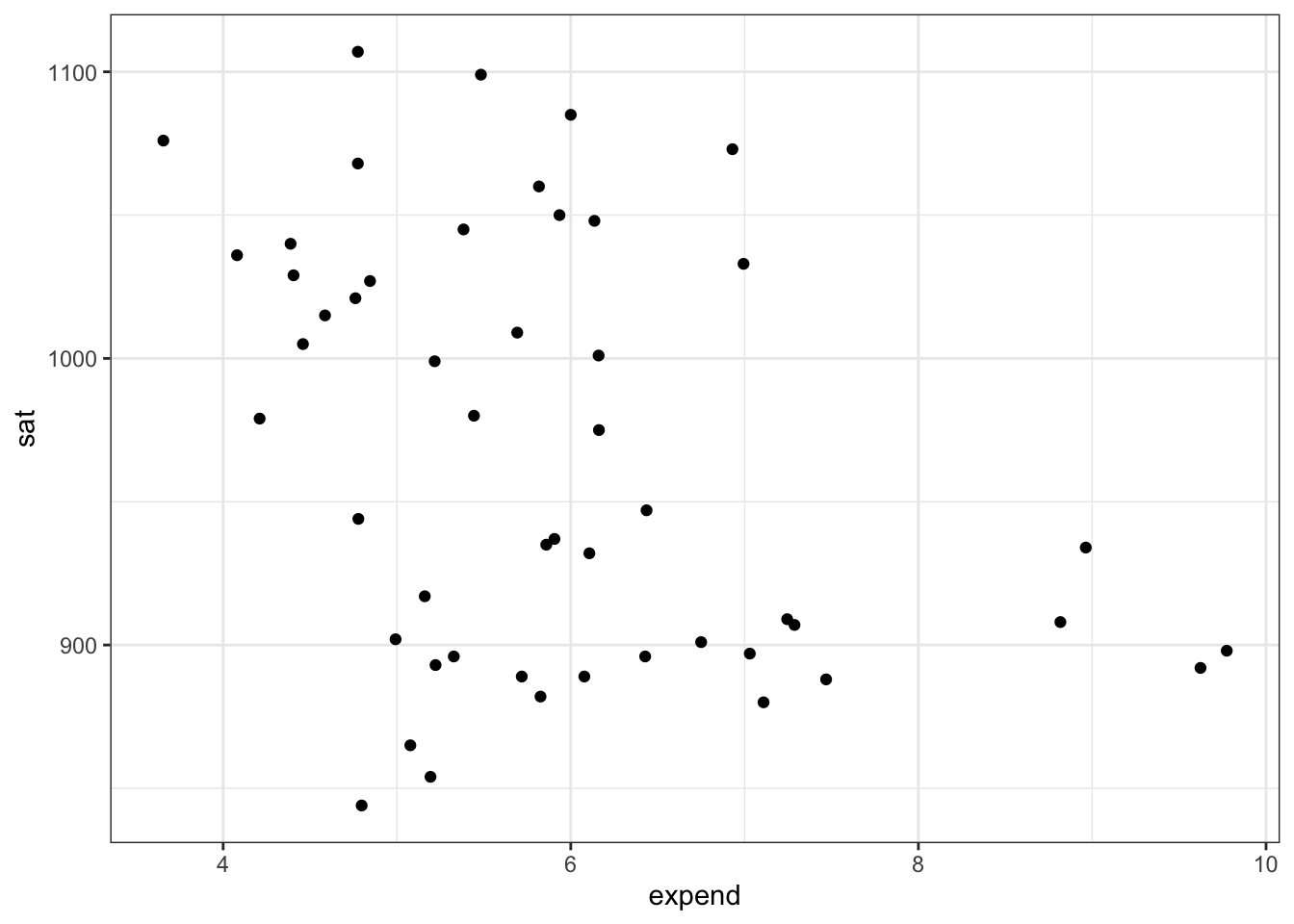
The SAT data set in the mosaicData package includes the following variables
for each state in the US:
sat– the average SAT score in 1994-95.expend– how much money was spent per student on education in 1994-94 (in thousands of US dollars), and
Design a simple linear model to predict the average SAT score from education expenditures in a state. Standardize variables where this is useful. Explain your choice of priors.
Now fit the model using
quap()and report a 95% HDI for the slope of your regression line (on the natural scale). What does this tell us about (what your model thinks about) SAT scores and education expenditures?Create a plot showing (a) the raw data, (b) a 95% HDI band for the predicted average average SAT score, (c) a 95% HDI band for the predicted “individual” average SAT score.
What is an “individual” in this data set? Explain why “average average” and “individual average” make sense in the previous problem.
6. More SAT.
Repeat as much of the previous problem as makes sense using a cubic B-spline with 4 knots.
For which state do the two models make the largest difference in prediction? How are you measuring “largest different in prediction”?
library(mosaicData)
gf_point(sat ~ expend, data = SAT)