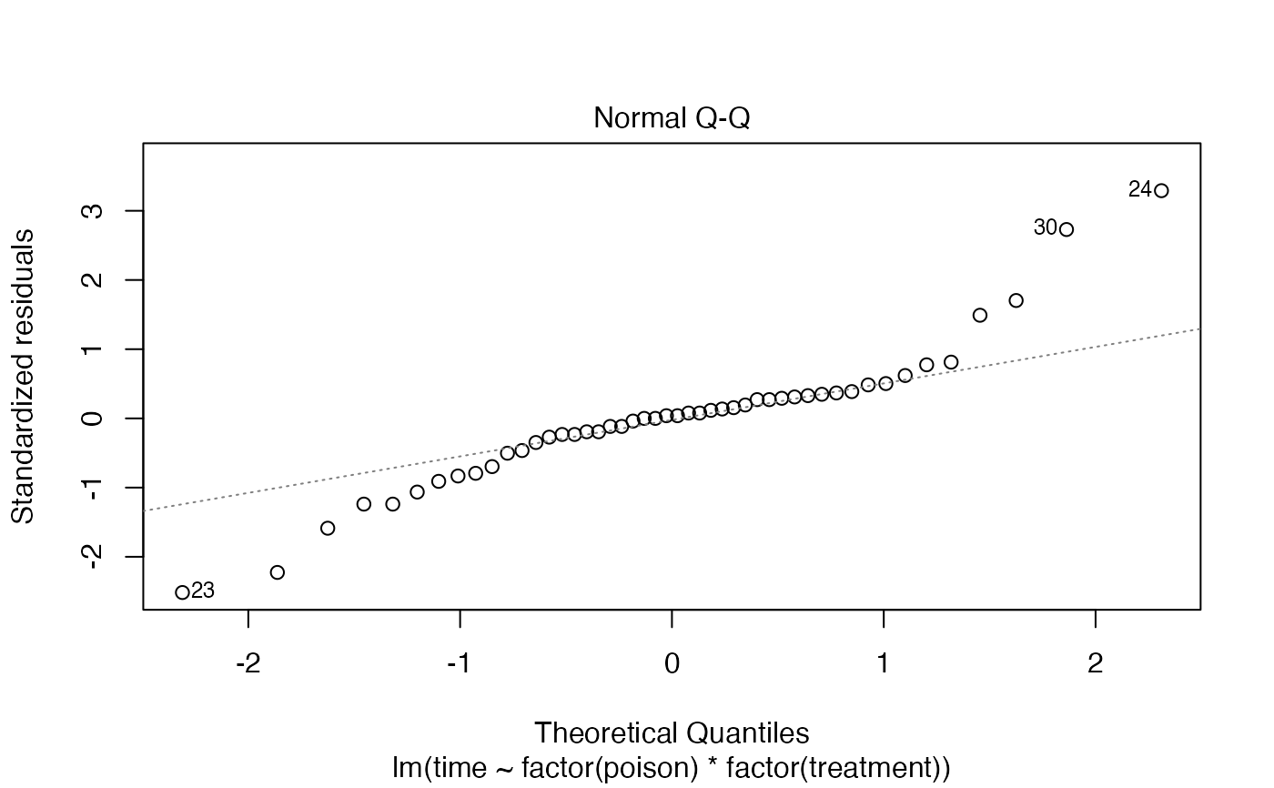
The data give the survival times (in hours) in a 3 x 4 factorial experiment, the factors being (a) three poisons and (b) four treatments. Each combination of the two factors is used for four animals. The allocation to animals is completely randomized.
Format
A data frame with 48 observations on the following 3 variables.
- poison
type of poison (1, 2, or 3)
- treatment
manner of treatment (1, 2, 3, or 4)
- time
time until death (hours)
Source
These data are also available from OzDASL, the Australian Data and Story Library (https://dasl.datadescription.com/). (Note: The time measurements of the data at OzDASL are in units of tens of hours.)
References
Box, G. E. P., and Cox, D. R. (1964). An analysis of transformations (with Discussion). J. R. Statist. Soc. B, 26, 211-252.
Aitkin, M. (1987). Modelling variance heterogeneity in normal regression using GLIM. Appl. Statist., 36, 332-339.
Smyth, G. K., and Verbyla, A. P. (1999). Adjusted likelihood methods for modelling dispersion in generalized linear models. Environmetrics 10, 696-709. http://www.statsci.org/smyth/pubs/ties98tr.html.
Examples
data(poison)
poison.lm <- lm(time~factor(poison) * factor(treatment), data = Poison)
plot(poison.lm,w = c(4,2))


anova(poison.lm)
#> Analysis of Variance Table
#>
#> Response: time
#>                                  Df  Sum Sq Mean Sq F value    Pr(>F)
#> factor(poison)                    2 103.301  51.651 23.2217 3.331e-07 ***
#> factor(treatment)                 3  92.121  30.707 13.8056 3.777e-06 ***
#> factor(poison):factor(treatment)  6  25.014   4.169  1.8743    0.1123
#> Residuals                        36  80.073   2.224
#> ---
#> Signif. codes:  0 ‘***’ 0.001 ‘**’ 0.01 ‘*’ 0.05 ‘.’ 0.1 ‘ ’ 1
# improved fit using a transformation
poison.lm2 <- lm(1/time ~ factor(poison) * factor(treatment), data = Poison)
plot(poison.lm2,w = c(4,2))


anova(poison.lm)
#> Analysis of Variance Table
#>
#> Response: time
#>                                  Df  Sum Sq Mean Sq F value    Pr(>F)
#> factor(poison)                    2 103.301  51.651 23.2217 3.331e-07 ***
#> factor(treatment)                 3  92.121  30.707 13.8056 3.777e-06 ***
#> factor(poison):factor(treatment)  6  25.014   4.169  1.8743    0.1123
#> Residuals                        36  80.073   2.224
#> ---
#> Signif. codes:  0 ‘***’ 0.001 ‘**’ 0.01 ‘*’ 0.05 ‘.’ 0.1 ‘ ’ 1